PRINCIPI DELLA DISTORSIONE DI FASE E STRUTTURA DI MODULAZIONE NON LINEARE
Nella prima parte di questo articolo, sono stati descritti i criteri e le metodologie utilizzati per la generazione del terreno e delle orbite di scansione. Questa seconda parte si concentra invece sull’implementazione del motore audio e sulla sua risposta ai dati estratti dalla superficie.
Il nucleo del sistema risiede in un algoritmo di Distorsione di Fase (Phase Distortion, o PD), una tecnica che consiste nel modificare l’andamento lineare della fase di un oscillatore prima che questa venga convertita in ampiezza da una funzione trigonometrica (come il seno o il coseno).
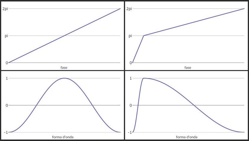
Nelle implementazioni classiche della distorsione di fase, l’andamento di un accumulatore di fase lineare (phasor) viene alterato in segmenti a pendenza variabile. Utilizzando la fase così distorta come indice di lettura per una lookup table, la forma d’onda originaria (tipicamente sinusoidale) subisce una deformazione geometrica che ne arricchisce lo spettro con parziali armoniche aggiuntive.
Diversamente dalle implementazioni tradizionali, in cui le variazioni delle pendenze sono guidate da inviluppi multi-stadio, il motore di distorsione di fase alla base di questo progetto viene modulato in tempo reale, utilizzando i valori estratti dalla scansione del terreno come coefficienti dinamici.
MAPPING DEL TERRENO E FUNZIONI DI TRASFERIMENTO
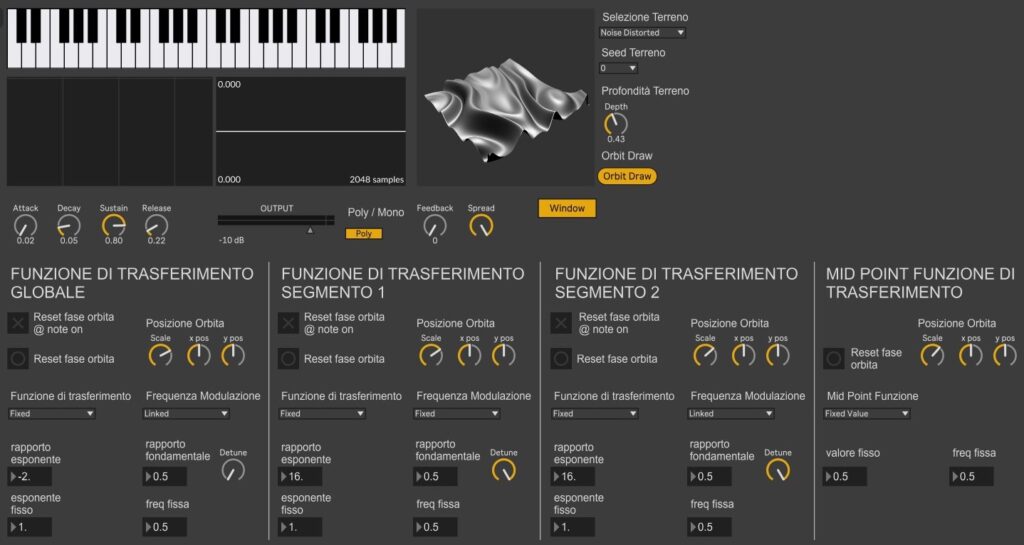
L’architettura del sistema si basa sulla flessibilità con cui i valori dell’asse del terreno intervengono sull’andamento della fase. All’interno del prototipo, l’ampiezza della superficie è normalizzata in un intervallo tra 0 (terreno piatto) e 1 (massima altezza). Le modalità con cui questi valori vengono riscalati definiscono l’esponente della funzione di trasferimento non lineare che rimodula il phasor prima della conversione trigonometrica. L’utente può selezionare tre diverse modalità operative, differenziate dall’intervallo in cui l’esponente viene mappato, per determinare il contenuto armonico risultante:
Esponenziale (esponente maggiore di 1)
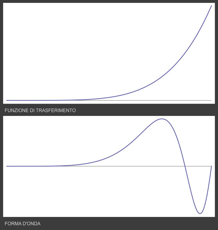
In questa configurazione, l’utente definisce un valore massimo di riscalamento superiore all’unità , determinando un andamento esponenziale per la funzione di trasferimento della fase. La rampa dell’accumulatore subisce una decelerazione iniziale seguita da un’accelerazione repentina in prossimità della fine del ciclo. Dal punto di vista spettrale, questa distorsione asimmetrica genera un arricchimento armonico progressivo e stabile, con un’estensione del contenuto in alta frequenza direttamente proporzionale ai valori estratti dal terreno.
Logaritmica (esponente frazionario)
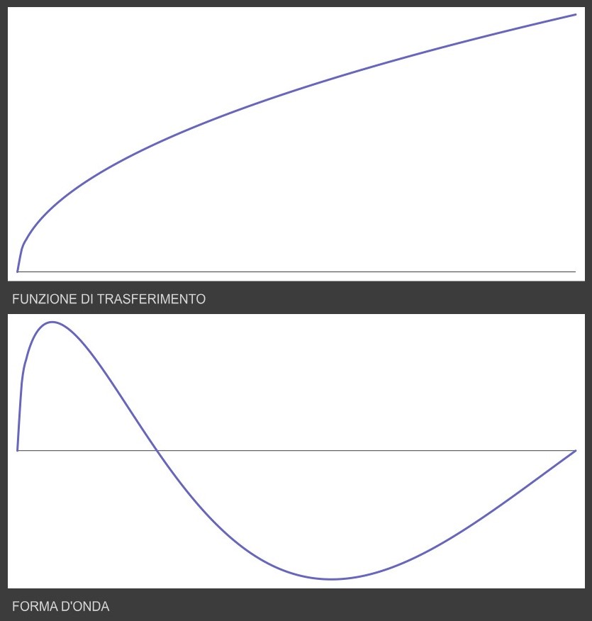
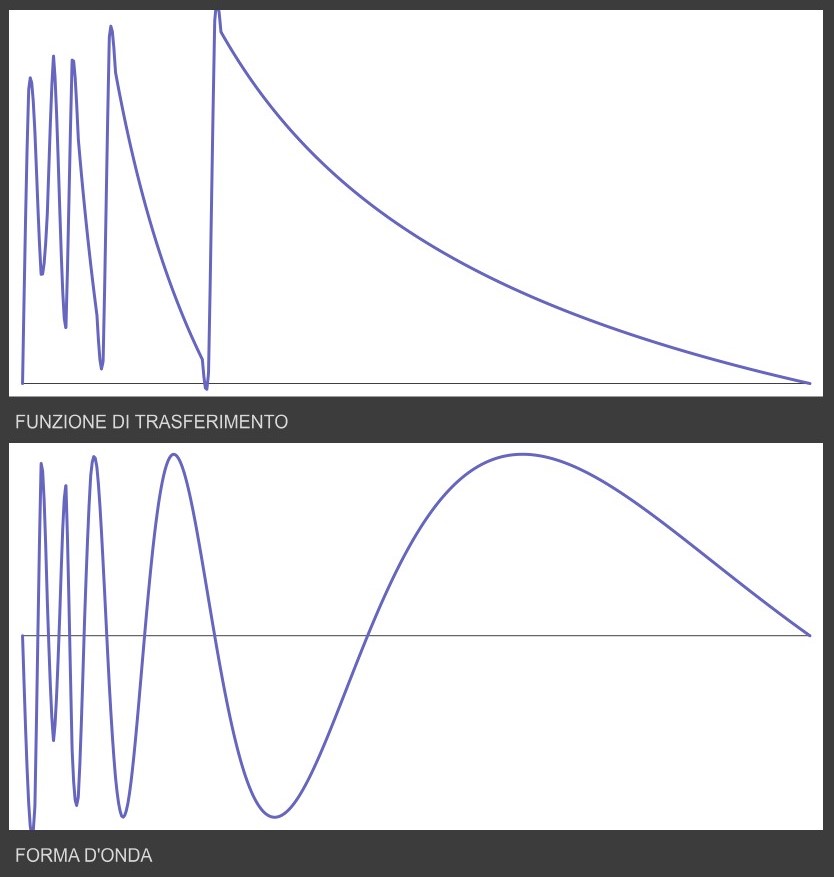
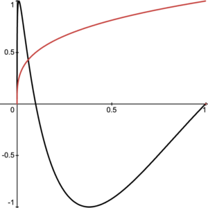
Limitando l’intervallo dell’esponente a una finestra frazionaria compresa tra 0 e 1, il sistema applica una distorsione di tipo logaritmico. La pendenza del phasor subisce una forte compressione geometrica, caratterizzata da una massima velocità di scansione all’inizio del ciclo e da uno spianamento successivo. Questo comportamento introduce una discontinuità netta nella transizione di fase che si traduce in uno spettro brillante e tagliente, con una forte presenza di componenti acute e parziali ad alta frequenza associate alla repentinità della deformazione iniziale.
Iperbolica (esponente negativo)
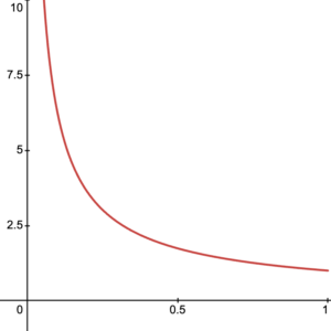
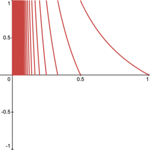
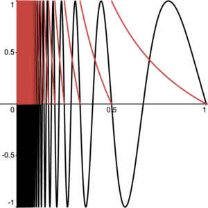
Mappando i dati del terreno in un intervallo di esponenti negativi , la funzione di trasferimento assume un andamento iperbolico estremamente ripido. Questa configurazione spinge i valori del ciclo di fase ben oltre la soglia nominale di 1; l’eccedenza viene ripiegata all’interno del dominio trigonometrico grazie alla periodicità della funzione seno. L’accumulo iperbolico in prossimità dello zero costringe il segnale a completare una fitta successione di cicli sinusoidali in una frazione ridotta di tempo. L’output audio risultante presenta uno spettro ad alta densità armonica e inarmonica, caratterizzato da fenomeni di intermodulazione e da una marcata ruvidezza timbrica dovuta alla forte non-linearità del sistema.
STRUTTURA DEL MOTORE AUDIO E CONTROLLO MULTIDIMENSIONALE DELLA FASE
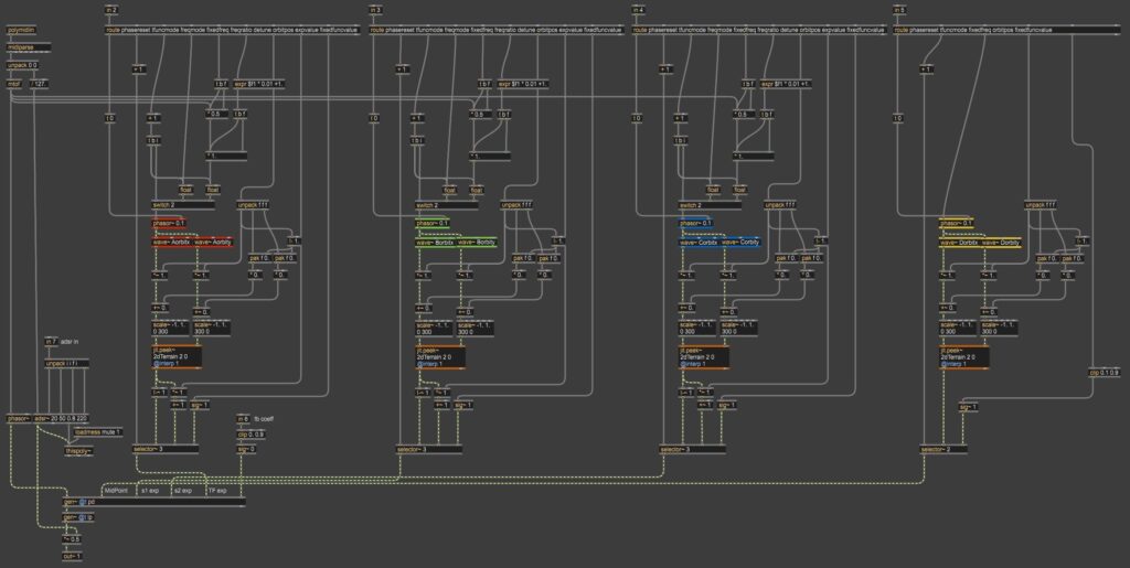
Il passaggio dal modello teorico alla generazione del segnale avviene attraverso un’architettura polifonica strutturata per mappare dinamicamente i flussi di controllo su ciascuna voce.
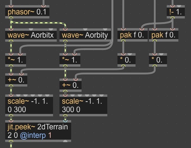
Ogni istanza include un accumulatore principale (phasor~) dedicato alla generazione della rampa lineare associata alla frequenza fondamentale. Per controllare i parametri del motore di sintesi, ciascuna voce gestisce quattro orbite di scansione simultanee e reciprocamente indipendenti.
Ogni orbita dispone di una coppia di oscillatori in quadratura e di un rispettivo oggetto di lettura (jit.peek~) interfacciato con la matrice globale del terreno. Questa indipendenza permette di configurare la velocità e la traiettoria di ogni scansione secondo due modalità principali:
Rapporto di Frequenza (Ratio): Un fattore di moltiplicazione calcola la frequenza dell’orbita in proporzione alla frequenza fondamentale della nota MIDI intercettata al Note-On.
Frequenza Fissa (LFO Mode): Gli oscillatori dell’orbita operano su un valore in Hertz svincolato dall’altezza della nota suonata, introducendo modulazioni spettrali asincrone.
I quattro flussi audio estratti dai rispettivi oggetti jit.peek~ governano in modo non lineare la geometria della fase del phasor~ principale prima dello stadio di conversione trigonometrica.
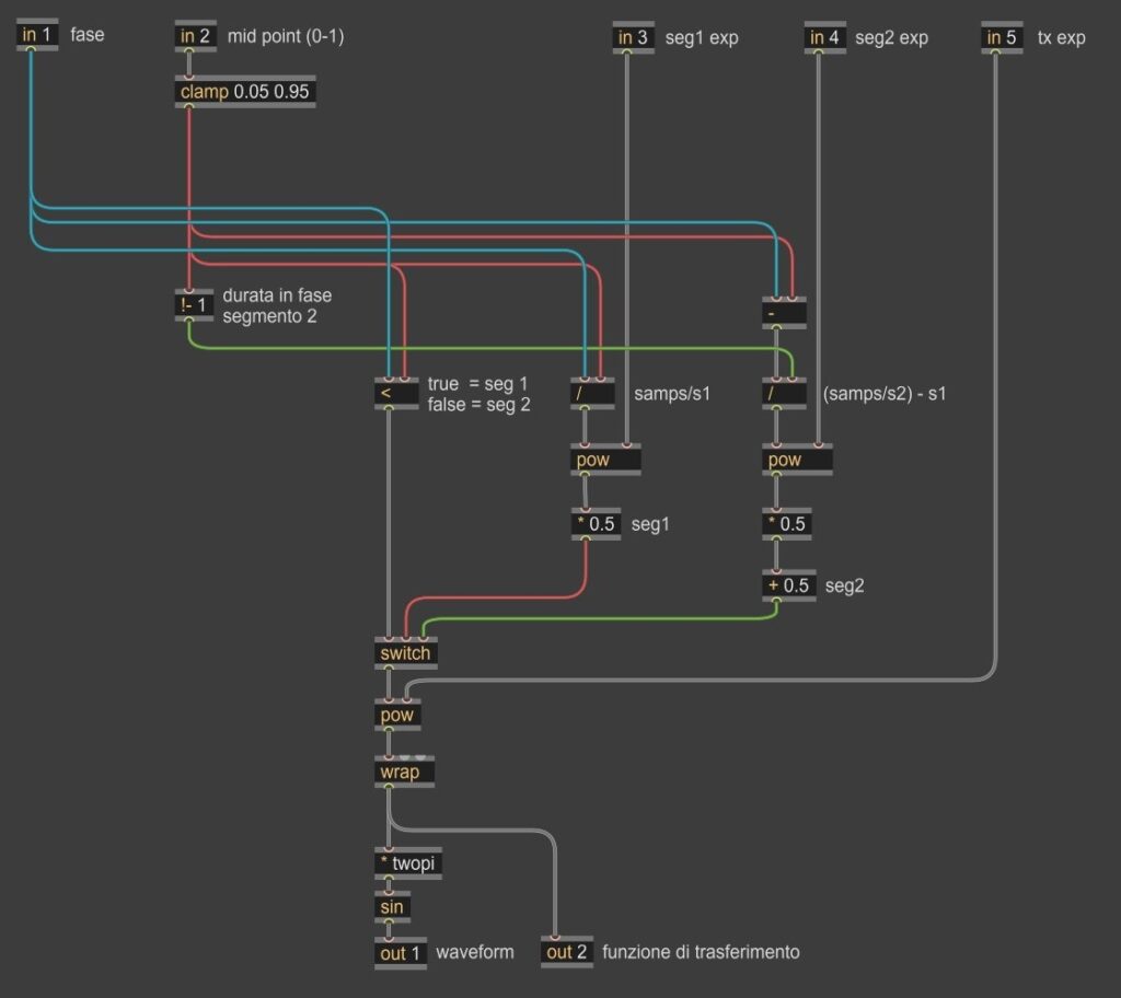
Il motore di distorsione segmenta la rampa lineare attraverso un punto di sfasamento intermedio, denominato midpoint, che suddivide il ciclo in due porzioni discrete. I flussi provenienti dalle quattro orbite di scansione vengono quindi destinati al controllo diretto dei parametri strutturali del sistema:
Esponente globale (Orbita 1): Modula la pendenza della fase sull’intero andamento della funzione di trasferimento.
Esponente del segmento inferiore (Orbita 2): Interviene sulla pendenza della fase nell’intervallo compreso tra lo zero e il midpoint.
Esponente del segmento superiore (Orbita 3): Interviene sulla pendenza della fase nell’intervallo compreso tra il midpoint e l’apice del ciclo.
Posizione del midpoint (Orbita 4): Determina il punto del ciclo in cui si attiva la transizione tra il segmento inferiore e quello superiore.
Grazie a questa configurazione, l’azione di ciascuna orbita sulla superficie a velocità differenti e con logiche di frequenza indipendenti produce una deformazione continua e asincrona della funzione di trasferimento. Questo approccio garantisce che ogni nota all’interno della polifonia mantenga la propria indipendenza armonica, pur preservando un’evoluzione spettrale coerente.
L’elaborazione in tempo reale di funzioni non lineari ad audio-rate, combinata con il campionamento simultaneo delle matrici tramite quattro oggetti jit.peek~ per ciascuna istanza, comporta un carico computazionale significativo in scenari polifonici densi. Per garantire l’efficienza del sistema, l’architettura adotta la procedura standard di gestione dinamica delle risorse prevista dall’ambiente Max/MSP, escludendo dal flusso computazionale le voci in fase di riposo e stabilizzando il consumo di CPU in proporzione diretta al numero di note effettivamente attive.
CONCLUSIONI E SVILUPPI FUTURI
Il prototipo sviluppato in questa fase iniziale dimostra la validità dell’integrazione tra la Wave Terrain Synthesis e il motore di distorsione di fase, estendendo le potenzialità espressive di entrambe le tecniche tramite lo spostamento funzionale del terreno da generatore d’onda a sorgente di controllo non lineare.
La flessibilità del mapping degli esponenti ha permesso di esplorare risposte spettrali complesse, gettando le basi per lo sviluppo di un sistema di sintesi versatile e capace di generare timbri dinamici e articolati.
I risultati ottenuti costituiscono una solida base per le fasi successive della ricerca. I futuri sviluppi si concentreranno sull’ottimizzazione del codice e sulla transizione del sistema verso un’architettura software definitiva. L’obiettivo a lungo termine prevede l’ingegnerizzazione dell’algoritmo per la distribuzione all’interno dei flussi di produzione musicale sotto forma di dispositivo Max for Live (M4L) o plug-in VST.
Come già visto nell’articolo introduttivo al progetto di ricerca, la Wave Terrain Synthesis (WTS) è una tecnica di sintesi basata sull’esplorazione bidimensionale di uno spazio geometrico. Un puntatore, seguendo una traiettoria, scansiona una superficie definita da una funzione a due variabili , dove i valori di ampiezza estratti lungo l’asse determinano l’andamento del segnale.
Nella sua implementazione classica, tuttavia, la corrispondenza diretta tra la conformazione del terreno e l’ampiezza dell’onda acustica limita la flessibilità timbrica del sistema, vincolando strettamente lo spettro risultante alla morfologia della superficie e alla frequenza di scansione.
L’obbiettivo di questo progetto di ricerca è estendere le potenzialità timbriche di questa architettura, esplorando le possibilità offerte dalla WTS come dominio di controllo dinamico e non lineare ad audio rate. All’interno del modello proposto, i dati estratti dall’esplorazione della superficie non generano direttamente il segnale audio; essi vengono invece interpretati e mappati per modulare in tempo reale i parametri e le funzioni di trasferimento di un motore a distorsione di fase.
TERRENO PROCEDURALE
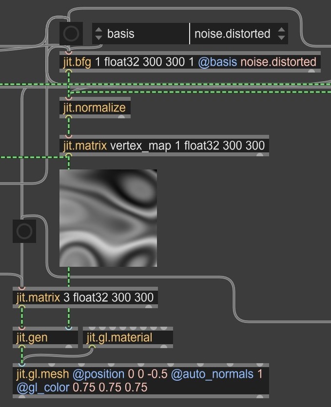
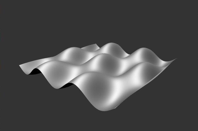
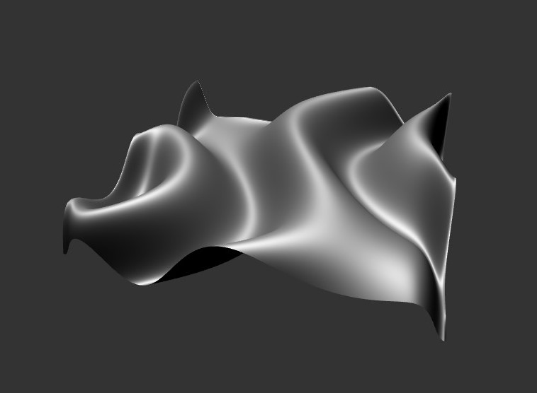
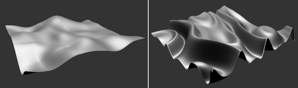
Nelle prime fasi di sviluppo del prototipo, la necessità primaria è stata quella di testare le potenzialità espressive del sistema su superfici complesse e non lineari. Invece di ricorrere a funzioni periodiche o a file pre-renderizzati, l’architettura della patch sfrutta l’oggetto nativo jit.bfg (Basis Function Generator) per calcolare frattali, rumori procedurali e funzioni ad alta variabilità, garantendo ambienti morfologici articolati e asimmetrici.
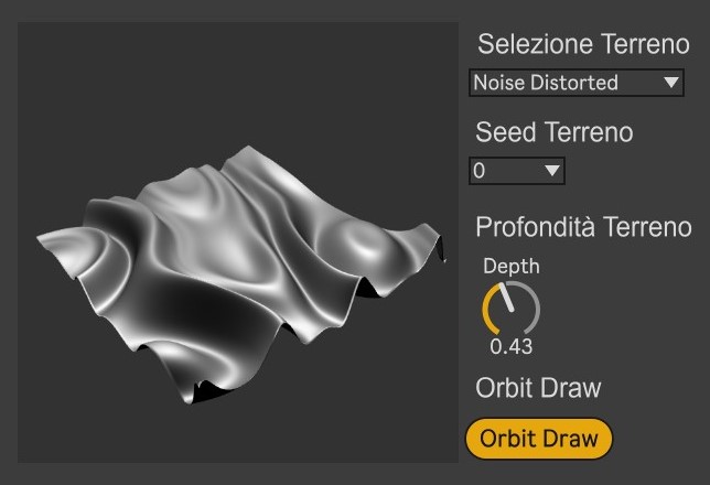
Per consentire all’esecutore di visualizzare in maniera più chiara la complessità dello spazio di controllo, il prototipo implementa un sistema di rendering tridimensionale in tempo reale. L’oggetto jit.bfg è configurato per generare una matrice bidimensionale a singolo piano, dove il valore di ogni cella rappresenta l’altezza (l’asse ) di quel punto nello spazio. Questa matrice viene elaborata come una vertex map e inviata all’oggetto jit.gl.mesh. All’interno del contesto OpenGL di Max, i dati bidimensionali della matrice vengono modellati nello spazio tridimensionale.
L’utente si trova così davanti a un panorama geometrico 3D che si deforma in sincrono con le modifiche ai parametri della funzione, rendendo immediatamente percettibile la relazione tra la topografia visiva e la risposta acustica del sistema.
Sebbene le prime versioni del prototipo includessero un modulo statistico basato su catene di Markov per automatizzare le transizioni tra le diverse funzioni morfologiche del terreno, questa architettura non è stata implementata nella release qui documentata. La decisione è derivata dalle repentine mutazioni del modello stocastico, le quali generavano un’eccessiva instabilità spettrale ad audio rate, evidenziando la necessità di un controllo più circoscritto e prevedibile sulla topografia della superficie.
ORBITE TRADIZIONALI E VETTORIALI
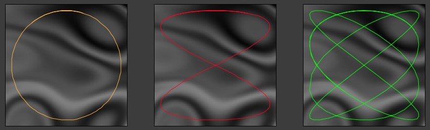
Un aspetto centrale della Wave Terrain Synthesis è la traiettoria seguita dal puntatore. Tradizionalmente, la scansione del terreno avviene tramite orbite geometriche regolari e periodiche: cerchi, ellissi o curve di Lissajous.
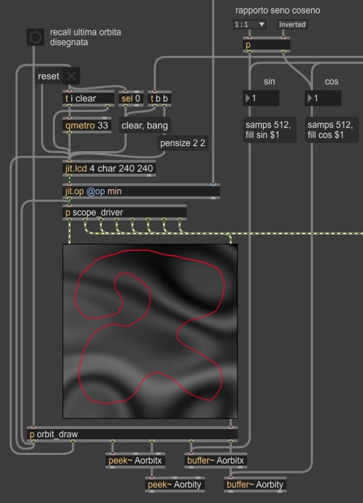
Per espandere le possibilità espressive del sistema, il prototipo introduce un’ulteriore modalità di interazione: la generazione di orbite vettoriali disegnate manualmente. Non si tratta della sostituzione dei modelli standard, i quali restano implementati nel sistema, ma di un’estensione gestuale che permette di confrontare il rigore e la precisione delle curve tradizionali con la fluidità e l’organicità del disegno umano.
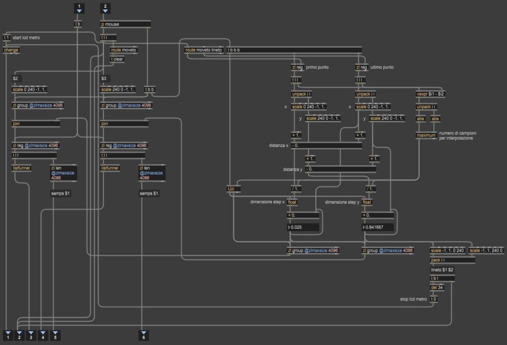
L’interfaccia di cattura è implementata tramite una subpatch, all’interno della quale l’utente disegna una traiettoria a mano libera all’interno dello spazio bidimensionale di un oggetto jit.lcd. Un algoritmo di parsing intercetta i movimenti del mouse, registrando le traiettorie, le accelerazioni e le decelerazioni del gesto. Il flusso di dati viene quindi scritto all’interno di una coppia di buffer audio, contenenti le coordinate spaziali e . Una volta memorizzata l’orbita bidimensionale, la lettura viene eseguita da una coppia di oscillatori audio rate. Questo garantisce una eccellente stabilità e permette di scansionare e modulare la velocità dell’orbita con la massima precisione.
Poiché il tracciato viene eseguito manualmente, il primo e l’ultimo punto definiti dall’utente non coincideranno quasi mai nello spazio bidimensionale. Dal momento che questi dati verranno letti in ciclo continuo dagli oscillatori, questa discontinuità geometrica creerebbe un salto repentino di coordinate a ogni fine ciclo, provocando click indesiderati. Per ovviare a questo problema, i dati passano attraverso una logica di interpolazione che collega linearmente le coordinate finali con quelle iniziali. Questo processo “chiude” l’orbita, garantendo una perfetta periodicità del ciclo di scansione e una riproduzione audio fluida e priva di artefatti transitori.
CAMPIONAMENTO DEL TERRENO E POLIFONIA
Il campionamento dei dati del terreno avviene all’interno di un ambiente polifonico gestito attraverso una subpatch poly~. La matrice bidimensionale generata dall’oggetto jit.bfg nella patch principale viene passata come riferimento condiviso a ciascuna istanza di poly~, dove l’oggetto jit.peek~ estrae il valore dell’altezza del terreno alle coordinate ricevute dagli oscillatori dell’orbita.
L’implementazione del campionamento all’interno dell’ambiente polifonico consente a ciascuna voce di generare traiettorie a frequenze indipendenti. L’utente può infatti vincolare la frequenza degli oscillatori di scansione a un rapporto di proporzionalità diretta con la frequenza fondamentale della nota MIDI in ingresso, oppure svincolarla per operare a bassa frequenza (LFO), estendendo le possibilità di modulazione.
Il segnale audio risultante dall’estrazione effettuata da jit.peek~ costituisce il modulo di controllo per il motore di distorsione di fase, il quale è in grado di operare con diverse curve di trasferimento (esponenziale, logaritmica, iperbolica), permettendo una modulazione non lineare dell’indice di distorsione guidata direttamente dalla topografia del terreno.
Il machine learning possiede una storia lunga e complessa, che precede di molti decenni l’attuale sviluppo dell’intelligenza artificiale generativa.
Nel corso della sua evoluzione il termine ha assunto significati differenti, accompagnando trasformazioni teoriche e tecnologiche che ne hanno progressivamente ampliato il campo di applicazione.
Questo articolo nasce anche da una riflessione maturata nel corso delle attività del nostro Dottorato di Ricerca. Negli ultimi due anni abbiamo progressivamente sviluppato una certa contrarietà nei confronti di quelle applicazioni del machine learning orientate alla progressiva sostituzione di alcune fondamentali prerogative dell’essere umano.
È importante chiarire sin dall’inizio che tale contrarierà non riguarda il machine learning come disciplina scientifica, né tantomeno il suo impiego nella ricerca musicale. Essa riguarda esclusivamente quelle interpretazioni radicali che attribuiscono alla macchina un ruolo progressivamente sostitutivo della volontà, della responsabilità e della creatività dell’essere umano.
Analoga perplessità suscita quella parte della ricerca contemporanea che tenta di demandare ai sistemi artificiali funzioni tradizionalmente appartenenti alla sfera umana, come il riconoscimento, la simulazione o perfino la generazione delle emozioni, prospettiva frequentemente ricondotta all’ambito dell’affective computing. Pur riconoscendone l’interesse scientifico, riteniamo che tali approcci pongano interrogativi etici e culturali che meritano un’attenta riflessione, soprattutto quando vengono applicati ai processi artistici e musicali.
La posizione qui proposta non si fonda quindi su un rifiuto della tecnologia, bensì sul rifiuto di ogni forma di radicalismo tecnologico che rischi di relegare l’essere umano a un ruolo marginale nel processo creativo.
Al contrario, riteniamo che il machine learning possa rappresentare uno strumento di straordinaria utilità quando venga concepito come supporto alle capacità del compositore, del ricercatore e dell’interprete, senza mai sostituirne le decisioni artistiche.
In questo senso, più che proporre una nuova definizione della disciplina, intendiamo presentare quello che potremmo definire un guided approach to machine learning: una prospettiva metodologica nella quale l’apprendimento automatico rimane costantemente guidato dagli obiettivi, dai valori e dalla volontà dell’essere umano.
Le origini del Machine Learning
Per comprendere questa prospettiva è opportuno tornare alle origini del concetto.
L’espressione machine learning fu introdotta nel 1959 da Arthur Samuel, ricercatore di IBM e tra i pionieri dell’informatica moderna. Samuel sviluppò un programma capace di giocare a dama migliorando progressivamente le proprie prestazioni attraverso l’esperienza, senza che ogni possibile situazione fosse esplicitamente programmata.
L’idea era rivoluzionaria: una macchina poteva apprendere dai dati e modificare il proprio comportamento nel tempo.
È importante osservare come, in quella fase storica, il machine learning avesse ben poco a che vedere con ciò che oggi viene comunemente definito intelligenza artificiale. Le grandi reti neurali, i modelli linguistici, gli algoritmi generativi e gli attuali sistemi conversazionali erano ancora lontani diversi decenni.
Il problema scientifico affrontato da Samuel consisteva soprattutto nello studio dei meccanismi dell’apprendimento automatico e nella possibilità di costruire programmi capaci di migliorare progressivamente le proprie prestazioni.
L’evoluzione del concetto
Durante gli anni Sessanta e Settanta il machine learning si sviluppò principalmente nell’ambito del riconoscimento di pattern, della classificazione automatica e dell’apprendimento statistico.
Negli anni Ottanta e Novanta la disciplina si arricchì con reti neurali artificiali, alberi decisionali, algoritmi genetici, macchine a vettori di supporto e numerose altre metodologie.
Solo negli ultimi quindici anni, grazie all’enorme disponibilità di dati e alla crescente potenza di calcolo, il machine learning è divenuto uno degli strumenti fondamentali dell’intelligenza artificiale contemporanea.
Questa ricostruzione storica mostra chiaramente come il machine learning non coincida con una singola tecnologia né con un’unica filosofia progettuale. Si tratta, piuttosto, di un insieme estremamente articolato di metodologie, suscettibili ancora oggi di interpretazioni profondamente differenti.
È proprio questa pluralità di significati che rende possibile elaborare approcci alternativi rispetto a quelli maggiormente diffusi nel dibattito contemporaneo.
Delega del processo creativo e affective computing
Nel panorama scientifico e artistico contemporaneo, l’applicazione del machine learning alla musica si muove prevalentemente lungo due direttrici che tendono a ridimensionare il ruolo dell’autore.
Da un lato, si assiste alla proliferazione di modelli generativi end-to-end, concepiti per produrre un output musicale finito a partire da un semplice input testuale o da un database di addestramento. In questo scenario, l’intervento umano si riduce spesso alla mera selezione o alla post-produzione di un materiale interamente strutturato dalla macchina.
Dall’altro lato, filoni di ricerca come l’affective computing tentano di formalizzare e mappare la complessa relazione tra strutture sonore ed emozioni umane, delegando agli algoritmi il compito di riconoscere o persino ottimizzare l’impatto emotivo di una composizione. Questo orientamento sottende l’idea che la risposta estetica possa essere interamente quantificata e, di conseguenza, ingegnerizzata.
È precisamente dinanzi a questa tendenza alla delega creativa e alla standardizzazione dei processi emotivi che si avverte l’esigenza di ridefinire i confini operativi della tecnologia nella ricerca musicale.
Un approccio guidato al Machine Learning
La prospettiva che proponiamo nasce proprio da questa consapevolezza. Se il machine learning costituisce una metodologia e non un fine, allora è possibile orientarne l’utilizzo secondo principi differenti.
Nel nostro caso il principio fondamentale consiste nella preservazione della centralità dell’essere umano. La macchina non rappresenta il soggetto del processo creativo, ma uno strumento progettato per ampliare le possibilità operative del compositore, del ricercatore e del musicista.
L’obiettivo non è automatizzare la creatività, bensì assisterla.
Più precisamente, riteniamo che il machine learning possa intervenire efficacemente nella risoluzione di problemi tecnici complessi, lasciando però all’essere umano ogni decisione estetica, artistica e progettuale. In questa prospettiva il rischio principale non consiste nell’utilizzo dell’intelligenza artificiale in quanto tale, bensì nell’eventuale progressiva delega delle decisioni creative alla macchina.
Per questa ragione il nostro interesse è rivolto a sistemi nei quali l’apprendimento automatico operi sempre entro limiti chiaramente definiti dall’autore del progetto, mantenendo la volontà umana quale riferimento costante dell’intero processo creativo.
Un esempio concreto
Questa impostazione trova una prima applicazione nel contesto del nostro dottorato di ricerca.
Il progetto riguarda lo sviluppo di nuove tecniche di sintesi sonora basate sull’integrazione tra wave terrain synthesis e phase distortion. In questo framework, il machine learning non viene impiegato per generare autonomamente materiale musicale né per sostituire il compositore nelle proprie scelte estetiche; al contrario, esso viene utilizzato come strumento di supporto tecnico.
Un esempio significativo riguarda il controllo delle complesse interazioni tra i parametri che regolano la risposta acustica del sistema. In presenza di particolari configurazioni, possono infatti manifestarsi instabilità numeriche o comportamenti indesiderati, gestibili tradizionalmente mediante regole rigide o istruzioni condizionali (if…then).
L’impiego del machine learning consente invece di apprendere, a partire da esempi selezionati dal ricercatore, modalità di comportamento più flessibili, adattando dinamicamente il sistema alle differenti condizioni operative. La scelta finale, gli obiettivi sonori e le decisioni artistiche rimangono interamente nelle mani del compositore.
Il caso di studio descritto risponde a una precisa scelta concettuale: rifiutare l’automazione del processo creativo per favorirne, invece, l’espansione. Mentre l’automazione mira a ridurre al minimo l’intervento umano per massimizzare l’efficienza produttiva della macchina, questa forma di integrazione si propone di potenziare le facoltà operative del musicista. In questo quadro, il machine learning perde qualsiasi pretesa di intenzionalità e si riappropria della sua natura originaria di strumento, i cui compiti si limitano all’ottimizzazione e alla gestione di variabili matematiche complesse o alla prevenzione di criticità strutturali.
È proprio questa, a nostro avviso, la direzione nella quale il machine learning può contribuire in modo più significativo alla ricerca musicale contemporanea, mantenendo la tecnologia al servizio della creatività e non viceversa.
Nel precedente articolo abbiamo notato come fase e frequenza siano strettamente legate tra loro. La fase, infatti, è proporzionale all’integrale della frequenza.
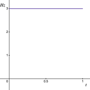
Prendiamo come esempio una frequenza di 3 Hz osservata però come un segnale costante:
Fig. 1 Frequenza costante di 3 Hz
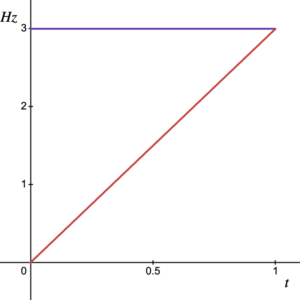
Ricostruiamone la fase calcolandone l’integrale:
Verrà fuori una retta inclinata da 0 a 3 in 1 secondo. Di norma sarebbe da 0 a , ma qui adottiamo una normalizzazione in cicli per praticità:
Fig. 2 Frequenza costante, in viola; fase risultante, in rosso
Ripercorriamo adesso lo stesso itinerario a ritroso: poiché la frequenza è la derivata della fase, applicando il calcolo della derivata alla retta inclinata di cui sopra, otterremo appunto la linea mostrata nella figura 1.
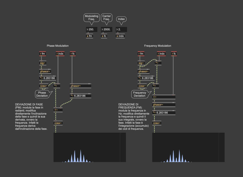
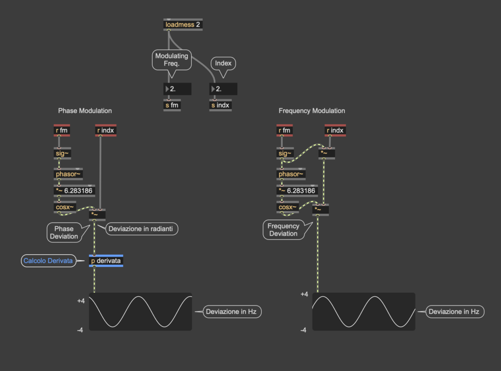
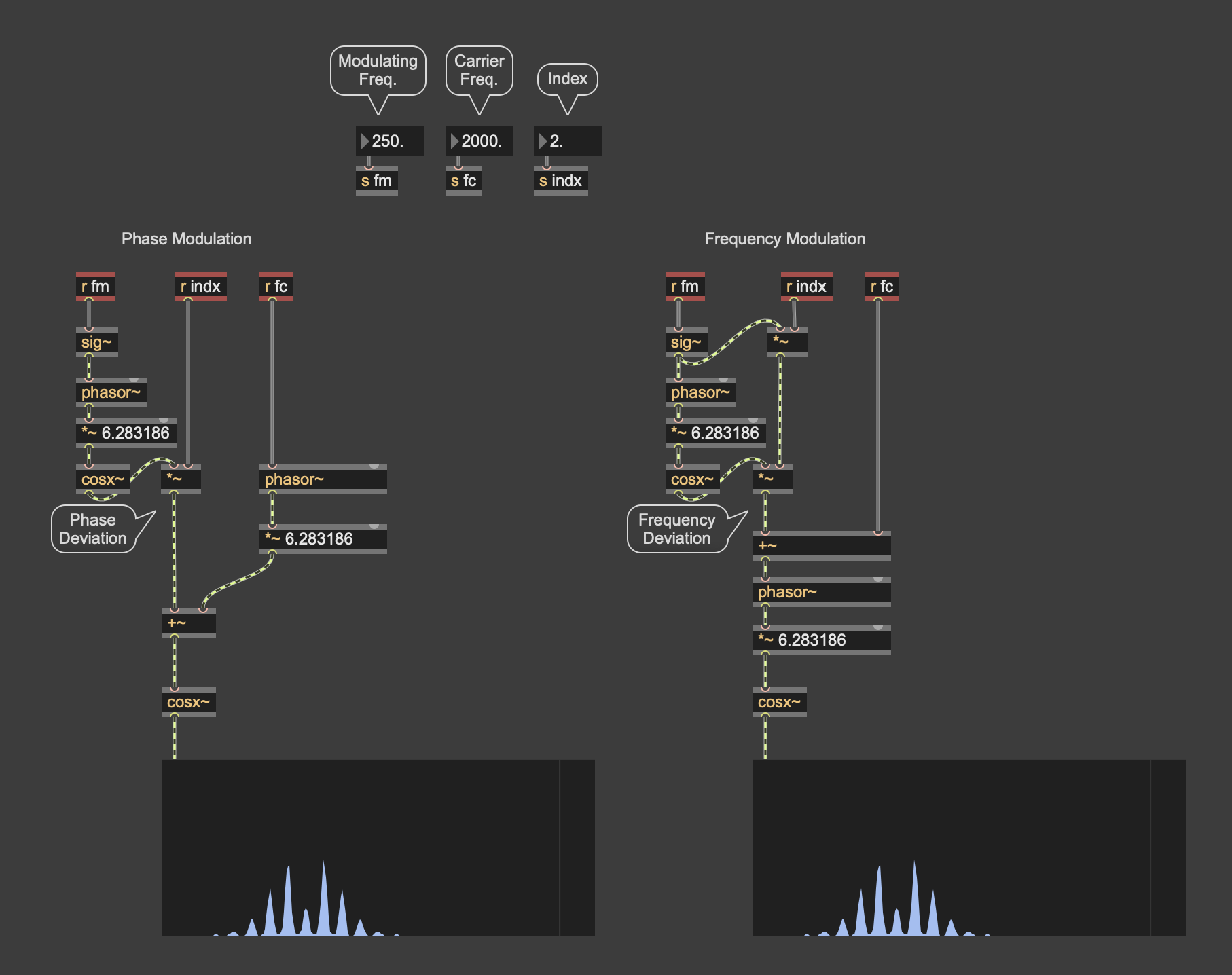
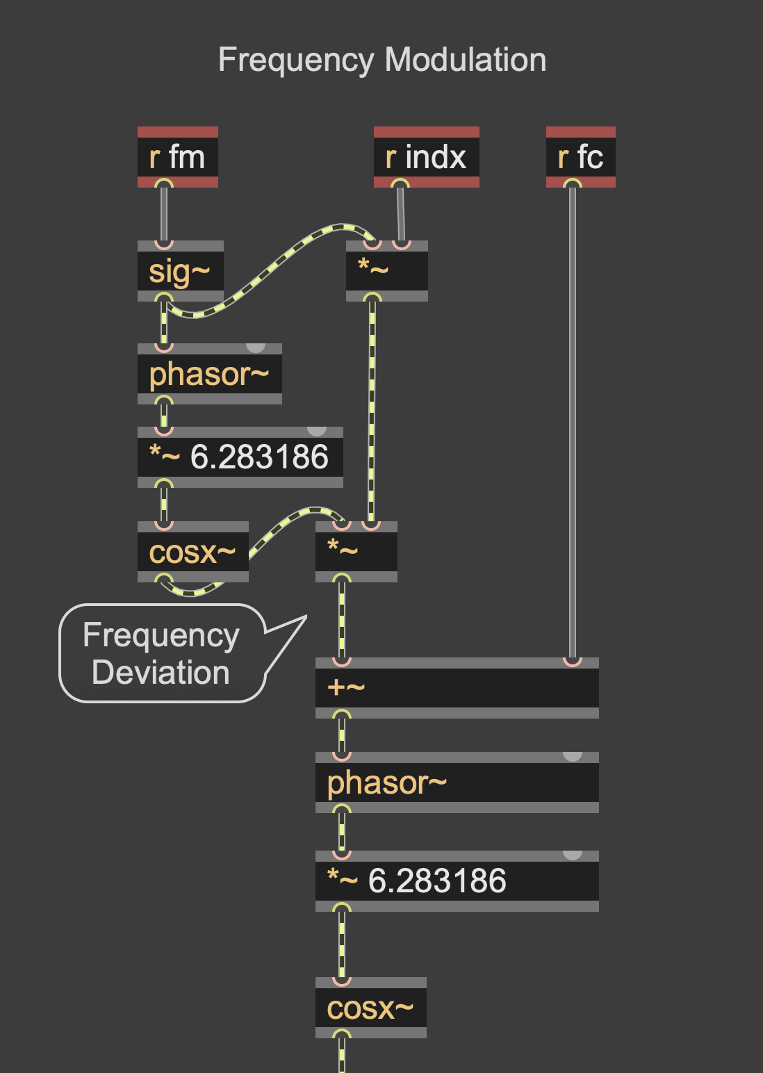
Queste premesse ci saranno utili per analizzare la patch qui di seguito riportata che mette a confronto Modulazione di Fase (PM) e Modulazione di Frequenza (FM):
Fig. 3 PM e FM hanno per modulante un segnale puro: gli spettri sono equivalenti
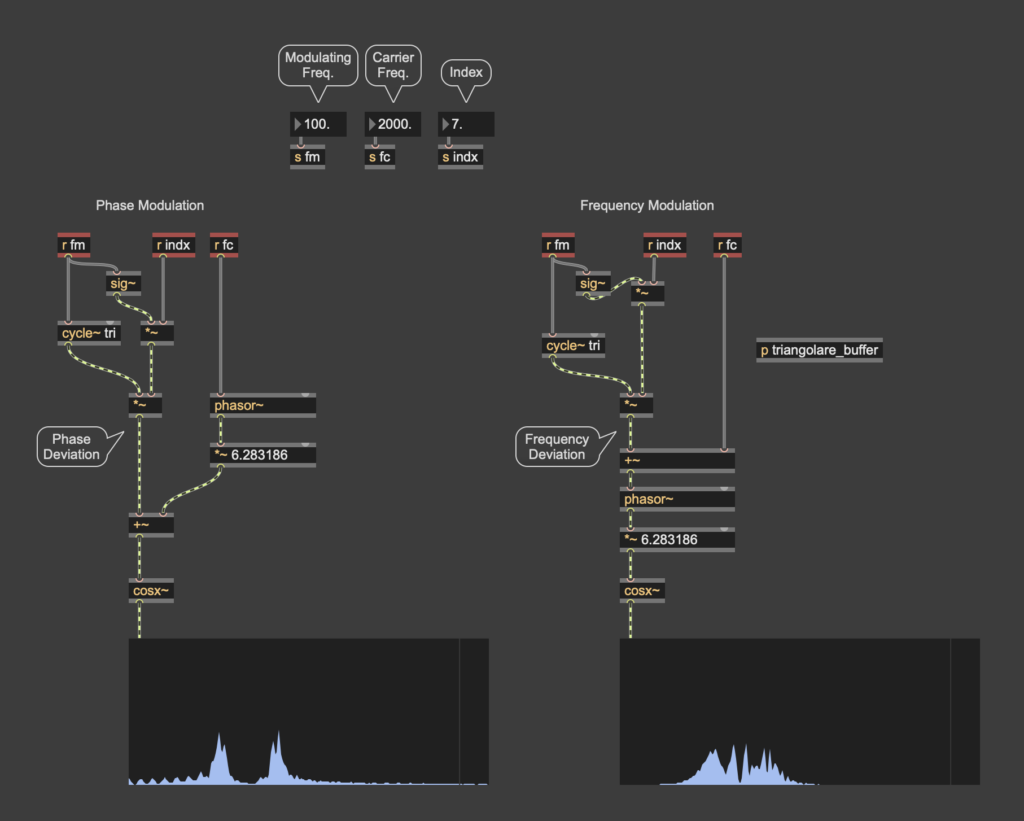
Fin quando nella modulante avremo segnali puri, sinusoidali (o cosinusoidali), le due modalità di sintesi rimarranno pressoché equivalenti. Nel caso in cui alla modulante daremo segnali non puri, i due spettri smetteranno di coincidere, come mostra la seguente figura 4, in cui alla modulante di PM ed FM è data un’onda triangolare:
Fig. 4 PM e FM hanno per modulante un segnale non sinusoidale: gli spettri non sono equivalenti
Nella PM mostrata nella figura 3, la modulazione è espressa in radianti. Se volessimo tradurla in termini di frequenza istantanea, dovremmo calcolarne la derivata, poiché la frequenza è proporzionale alla variazione della fase nel tempo:
Fig. 5 Segnali modulanti di PM e FM. Nella modulante della PM, l’output espresso in radianti è stato tradotto in frequenza istantanea tramite il calcolo della derivata
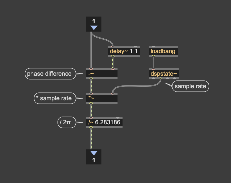
In ambito discreto, la derivata può essere ottenuta calcolando la differenza tra due campioni consecutivi della fase, moltiplicando il risultato per la frequenza di campionamento e dividendo infine per , così da convertire il valore in Hertz:
Fig. 6 Subpatch della patch in figura 5: calcolo della derivata
Applicando questo procedimento alla PM, si osserva che il risultato è pressoché equivalente all’onda mostrata nella sezione FM della figura 3. In altre parole, quando il segnale modulante è una sinusoide (o cosinusoide), la deviazione di frequenza ottenuta dalla derivata della PM coincide sostanzialmente con quella prodotta direttamente in una FM.
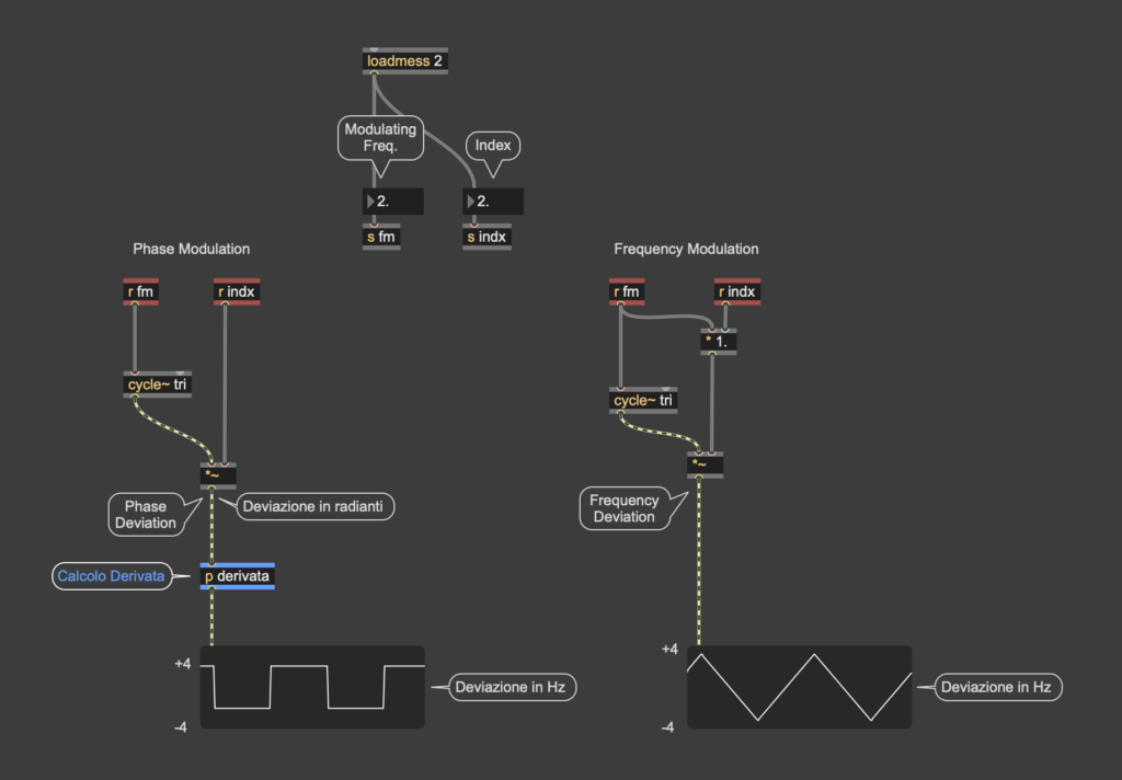
Come già detto, la situazione cambia se si utilizza una forma d’onda differente. Nella seguente figura 7 sono mostrate le sole modulanti triangolari di PM e FM. Calcolando la derivata della deviazione di fase, compare infatti un’onda quadra anziché una triangolare:
Fig. 7 Modulanti triangolari di PM e FM. Nella modulante della PM, l’output espresso in radianti è stato tradotto in frequenza istantanea tramite il calcolo della derivata, questa volta i segnali non sono affini, come avveniva invece nella figura 5.
Ciò avviene perché la derivata misura l’inclinazione della fase: nelle rampe ascendenti e discendenti della triangolare, l’inclinazione rimane costante, per cui il risultato non è una variazione graduale della frequenza, ma due livelli di frequenza costanti che si alternano bruscamente. La derivata della triangolare è quindi una forma d’onda quadra.
Nella sezione FM della patch 2, invece, la deviazione di frequenza mantiene la forma triangolare originale del segnale modulante. Questo esempio mostra chiaramente che l’equivalenza tra PM e FM rappresenta un caso particolare legato all’impiego di una modulante sinusoidale e non una proprietà valida per qualsiasi forma d’onda.
Un’ulteriore conseguenza di questa differenza emerge osservando gli spettri prodotti dalle due tecniche mostrati nella figura 4. Nel caso della patch con modulante triangolare, la PM infatti produce distribuzioni spettrali insolite, spesso caratterizzate dalla scomparsa di alcune componenti armoniche o dalla presenza di cancellazioni particolarmente marcate. Il risultato si discosta sensibilmente dalla classica PM sinusoidale descritta dalle funzioni di Bessel e può ricordare, in alcuni casi, una commutazione periodica tra due differenti deviazioni di frequenza. Tali comportamenti evidenziano ulteriormente come l’equivalenza tra PM e FM sia una proprietà specifica della modulazione sinusoidale e non possa essere estesa arbitrariamente ad altre forme d’onda.
A corollario di quanto espresso, possiamo aggiungere che non è raro che formule comunemente presentate come esempi di modulazione di frequenza siano in realtà modulazioni di fase. Una formula FM frequentemente riportata nei manuali è infatti:
Tuttavia, osservando attentamente l’espressione, si nota come la modulante venga sommata direttamente alla fase della portante. Ciò che viene modulato in maniera esplicita è dunque la fase e non la frequenza.
Nell’espressione , la quantità può essere infatti considerata come la traiettoria di fase dell’oscillatore. Per questo motivo, quando un termine di modulazione viene aggiunto all’interno dell’argomento della funzione sinusoidale, esso agisce di fatto sulla fase.
Una formula più esplicita di modulazione di frequenza potrebbe dunque essere:
Giusto per chiarezza esplicativa, dividiamo in due parti quest’ultima formula, vale a dire sezione portante:
e sezione modulante, cioè l’integrale della deviazione:
Dapprima si crea dunque una deviazione di frequenza che, per essere inserita in formula, viene convertita in fase calcolandone l’integrale.
Poiché richiede una fase espressa in radianti, occorre moltiplicare per affinché l’intera formula:
sia pressocché equivalente a:
Più che una distinzione rigida tra tecniche differenti, PM e FM mostrano dunque come la fase possa essere osservata da prospettive diverse: talvolta come quantità direttamente manipolata, talvolta come risultato dell’integrazione di una variazione di frequenza. Comprendere questa relazione significa acquisire uno strumento concettuale utile per osservare PM e FM non come tecniche indipendenti, ma come differenti punti di vista sul rapporto tra fase e frequenza.
The Max software, created by Miller Puckette and currently developed and distributed by Cycling ’74, was designed in the 1980s as a graphical programming environment for musical creation, and has since then been used in several other artistic domains. But as a programming environment, Max can also be used for non-creative purposes; this article presents how it can be used as a tool for the musicological investigation of the repertoire of computer music. After an introduction to software-based approaches to the study of such a repertoire, an extensive research project dedicated to nine case studies serves as a basis for the discussion of key aspects of developments using Max in a musicological context. In this paper, the focus is on the potential afforded by Max in such contexts rather than on the particular musicological investigations. Perspectives for a generalization of this approach are therefore proposed, considering the modules created in this project according to their specificity, generality, or potential for abstraction beyond the work that motivated them. This ultimately leads to a consideration of Max as a tool for musicological research and analysis beyond the field of computer music.
INTRODUCTION
A graphical programming environment, the Max application1 distributed by Cycling ’74 is primarily aimed at and used for artistic and in particular musical creation. Its first application was the complex interaction between piano and live electronics in Philippe Manoury’s Pluton (1988, final version 1989), and it is now used as a key element in the creative toolset of countless musicians and artists of very diverse backgrounds and aesthetics. Of the most recent 100 projects, at the time of writing this article, developed by Max users and displayed on Cycling ’74’s project page,2 93 can be deemed creative in that they are either artistic outputs or tools to be used in a production, composition, or performance context; 93 are of musical or audiovisual nature. Despite such a significant artistic scope, Max is sufficiently generic an environment for its users to develop non-creative artifacts. In the TaCEM project (Technology and Creativity in Electroacoustic Music), funded by the United Kingdom’s Arts and Humanities Research Council (AHRC) and led by the three authors of this article,3 Max was used as the primary programming environment to conduct and disseminate a research of musicological order: the analysis of the interaction between compositional or performance processes and technology in nine important works of computer music. This project resulted in a recently published book accompanied by a Mac/PC application for each of these nine case studies [1], all built from Max, and demonstration videos constituting a bridge between the written chapters and the software.4 How can Max be used as a tool for musicology and music analysis? The second section of this article presents the implications of software-based approaches for the study of musics which exists primarily as sound – as opposed to those which rely on the intermediary support of the score, which have been historically dominant in Western musicology5 – and in particular the repertoire of computer music. Key aspects of Max-based developments are then, in the third section, discussed on the basis of the experience gained through the authors’ TaCEM project, with implications on both the research itself and its dissemination. Within a consistent but heterogeneous repertoire, a variety of analytical needs have been identified and addressed, Max in some cases proving a natural toolbox, in other cases showing limitations but ultimately enabling very positive analytical outcomes. Finally, the fourth section of the article considers the overall research and development process of this project in the light of the notions of specificity, generality, and abstraction.
SOFTWARE-BASED APPROACHES TO MUSICOLOGY
Interactive aural analysis and reconstructive approaches to the computer music repertoire
Interactive aural analysis, developed by Michael Clarke for the study of electroacoustic music and formally presented in [3], is a musicological approach proposing a substantial integration of software into the analytical processes and outcomes, where “the reader is presented with tools with which to explore aspects of the music for themselves alongside the author’s suggested interpretations.”6 Such a software-based approach can be applied to the investigation of the techniques used by the composers in the studio, whether they operate on audio signals or higher level representations, and to the organization of the musical work as a whole. If “visual representations and words alone may not be the ideal means by which to present an analysis of electroacoustic music,”7 the interactivity enables the approach not only to provide access to dynamically-evolving processes, but also to integrate the aural at the heart of the analysis.
This interactive aural approach was first implemented by Clarke in 2006 for the analysis of Jonathan Harvey’s Mortuos Plango, Vivos Voco (1980), where the written article is accompanied with a software application on DVD [4] enabling the reader to engage with interactive aural examples for the exploration of the composer’s techniques and his approach to timbre, harmony, and structure. Another publication was later realized in 2010 for the issue of Ina-GRM’s Polychrome Portraits dedicated to Denis Smalley, with an interactive aural analysis of Wind Chimes (1992), here too combining a written chapter and a standalone application [5]. The following year, an ethnographic study of the creative process and performance of Michael Finnissy’s Second String Quartet (2007) was jointly published by Amanda Bayley and Michael Clarke [6] – unlike the previous two analyses, the publication was entirely in software and distributed on DVD. In 2012, the three authors of this article initiated a large investigation of the computer music repertoire8 with both a contextual and historical approach and the development of interactive aural analyses for nine case studies: John Chowning’s Stria (1977), Barry Truax’s Riverrun (1986), Philippe Manoury’s Pluton (1988/1989), Hildegard Westerkamp’s Beneath the Forest Floor (1992), Francis Dhomont’s Phonurgie (1998), Trevor Wishart’s Imago (2002), Jonathan Harvey’s Fourth String Quartet (2003), Cort Lippe’s Music for Tuba and Computer (2008), and Natasha Barrett’s Hidden Values (2012). This resulted in the publication of the aforementioned monograph [1] with nine standalone applications and 105 demonstration videos, key aspects of which are considered in terms of developments in the third section of this article.
The interactive aural approach is related to other initiatives where a software-based approach is fundamental in the implementation of the musicological scrutiny. In an article from 2003 [7], Marc Battier proposed the concept of faktura as “a conceptual tool for analysis [which] may lead to using the method of reverse engineering. In this technique, the analyst turns back and follows the composer’s inverse path, the path from the final work to the initial ideas and materials, a paradigm which hopefully leads one to a description of the processes involved in making the piece and the production of the sound material.”9 Several musicologists undertook such a reconstructive approach to the computer music repertoire: in a 2007 issue of the Computer Music Journal, both Kevin Dahan and Olivier Baudouin proposed independent reconstructions of Chowning’s Stria [8, 9]. In 2011, Andreas Bergsland presented his Six Fantasies Machine (SFM), a program producing a range of sound similar to those of Paul Lansky’s Six Fantasies on a Poem by Thomas Campion [10]. In 2016, Sean Williams proposed a similar approach – all in the analogue domain – to research interpretation and performance practice in Karlheinz Stockhausen’s Studie II (1954) [11], a piece which Joachim Heintz had also reconstructed in software [12]. Also relevant is Alain Bonardi’s software reconstructions of Philippe Manoury’s live electronics in En écho with both musicological and preservation oriented concerns [13].
Max as a tool beyond musical creation
In 2002, Miller Puckette defined Max as a paradigm: “I have worked for many years on a computer environment for realizing live electronic music that I named in honor of Max Mathews. Three currently supported computer programs – Max/MSP, jMax, and Pd [Pure Data] – can be considered as extended implementations of a common paradigm I refer to here as ‘Max’.”10 In this article, we consider the actual Max software (in 2002 known as Max/MSP). Its primary scope is that of musical creation, but as David Zicarelli, CEO of Cycling ’74, the company which develops and distributes Max, specified in 2018, “Max started in music, but it’s increasingly used in art and architecture [university] programs.”11 We consider here Max as a programming environment – not a language – although it is important to recognize that this is a frequent point of discussion in its community of users and developers.12 For instance, Puckette wrote that “musicians have often used Max as a programming environment, at which Max succeeds only very awkwardly. […] Rather than a programming environment, Max is fundamentally a system for scheduling real-time tasks and managing communication among them. Programming as such is better undertaken within the tasks than by building networks of existing tasks. This can be done by writing ‘externs’ in C or C++, or by importing entire interpreters.”13
Considering that programming encompasses both the construction of networks of objects using the visual paradigm of patching and the possibility of integrating the textual via, for example, C and JavaScript, it is straightforward to see Max as a tool that can have applications beyond artistic creation, and in a very generic way. For the focus of this article, namely musicology and the analysis of creative processes using technology, and in particular our TaCEM project, several dimensions made Max a promising initial candidate. Its musical and audio orientation, the existence of a large library of objects and in particular graphical user interface ones, the possibility to integrate C externals for message, signal, and matrix data, and the opportunity to create a fixed standalone for both Mac and PC, led us to use Max consistently throughout the project. The following quotation by Lippe and Settel perhaps best summarizes the balance we found: “Using this [external code resource] platform, it is possible to combine the power of C with the convenience and speed of Max […], and development time can be quite rapid”14. Indeed, any programming environment – visual or not, music and audio-oriented or not – can lend itself to the development of a software-based approach to the study of music. Among the musicological examples introduced in section 2.1 above, Max was used for all cases of interactive aural analysis, from Mortuos Plango to Inside Computer Music; Dahan used Ruby and Csound, Baudouin used Python and Csound. Csound was also used by Bergsland and Heintz; Bonardi used Faust. In the forthcoming and third section of this article, we describe in more detail key elements of our experience designing the Inside Computer Music software with Max.
MAX AS A TOOL FOR CONDUCTING AND DISSEMINATING RESEARCH
The emulation of historic environments and generic processes
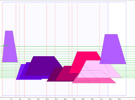
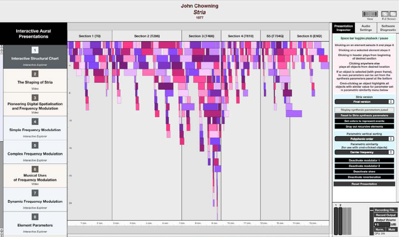
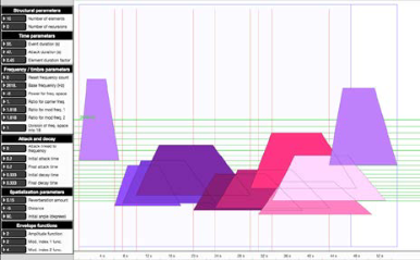
In order to give an understanding of the compositional environments and methods of the studied composers, we have, where potentially insightful and technically possible, undertaken their emulation. The first example of this was the investigation of John Chowning’s programs for Stria: the SAIL algorithm for the composition of event parameters – consistent sets of individual elements – was, following the aforementioned approaches in [8] and [9], replicated – here using JavaScript in a Max JSUI15 object enabling us to implement a fully interactive interface. In one of these interfaces, the user can experiment with the reproduction of the algorithm’s parameters of event structure, time, frequency, frequency modulation, and spatialization; the parametric changes are immediately visible graphically (figure 1) and the result audible (playback can operate on the event as a whole, or on individual elements; the reverberation can also be deactivated to focus on the sound of the dry frequency modulation).
Figure 1. Graphical representation of the first event of Chowning’s Stria in the software accompanying Inside Computer Music – each polygon represents one of the ten individual elements.
With a second interface, we reproduced the step-by-step command-line interface, where the result is only audible once all parameters have been entered by the user. In both cases, the audio was simply implemented, for the two modulator / one carrier algorithm and the reverberation, with plain MSP16 objects, approaching the original MUSIC 10 synthesis design.17
Another emulation was that of GSX, the real-time system Barry Truax developed for granular synthesis, and used in his landmark work Riverrun. Like with Chowning, the publicly available documentation on the subject is excellent, enabling us to develop a first prototype – again, with a simple user interface using the JSUI object, in order to approximate Truax’s own terminal, and MSP objects, with custom C externals designed to trigger the grains specifically18. In this case, some further discussion with the composer and fine-tuning work alongside his original system was necessary, but our attempt was eventually successful at simulating the behavior of GSX.19
Studying Francis Dhomont’s Phonurgie, the opportunity to develop a simple model of Ina-GRM’s SYTER, the institute’s first real-time audio digital environment [19] developed as it became apparent that it had been extensively used by the composer for this piece and several others. Here, the motivation was not to reproduce exact materials, but to give the user – and indeed ourselves, as researchers – a better sense of the interaction with this environment. On the basis of available documents on the system,20 we reproduced the fundamentals of the user interface using a JSUI object and some audio processors in plain MSP objects. The scope of the project did not permit us to attempt a full emulation, but our final prototype gives a good account of the user interaction with the system, especially the interpolation ‘balls’ which enable all the parameters to be modified at once by navigating a two-dimensional screen between memorized presets, very much like the current Max nodes object. In some cases, the implementation of generic techniques was sufficient to give a precise account of the composer’s process. Composing Beneath the Forest Floor, Hildegard Westerkamp experimented with field recordings and digital modules such as time-domain gating, speed variation resulting in transposition, delay, harmonization, reverse playback, or reverberation. Without knowledge of the specific implementation of those actually used, but with access to the composer’s archive of sound files for the work,21 generic implementations of such techniques proved useful in approaching the composer’s materials. These were implemented using standard MSP objects, with an external specifically developed for flexible playback with continuous signal rate speed control, including backwards, and looping, in conjunction with the TaCEM playback user interface. Studying Wishart’s Imago, a number of non-real-time processors, including several involving FFT and phase vocoding, were also implemented generically, which proved sufficient to give a detailed account of much of the composer’s creative process.22
Musicological refactorization of Max performance patches
Where Max is used as part of the creative process of a work being researched, using Max as environment for the analysis naturally facilitates the investigation; where the interactivity between performer and electronics relies on a patch, one can consider the electronic instrument as the direct subject of analysis [21]. In the TaCEM project, this was the case with Manoury, Harvey, Lippe, with different aesthetics, instruments (respectively piano, string quartet, and tuba), and interaction modes, but with a general patch architecture typical of IRCAM with the audio modules grouped in a “DSP” subpatch, and parameters controlled by sending event-tagged messages from qlist objects.
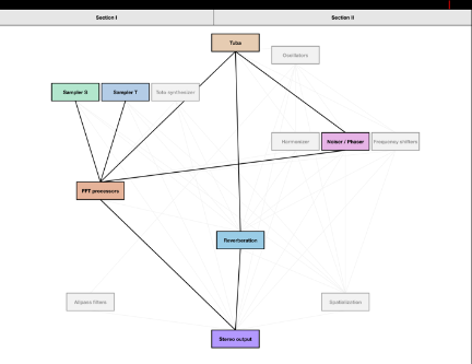
The performance patches are complex and, although logically organized and of course operational for performance purposes, they are difficult to scrutinize as is with musicological intentions. Our approach was first to try to extract each audio module, simple or complex, and make it available for independent exploration – in order to understand its expressive and aural potential outside the context of the work itself. This had been done with several interactive examples in a CD-ROM on Manoury’s works for real-time electronics [22]; in TaCEM, we systematized the approach to all available modules and parameters. The next step was then to understand – and communicate – how these modules where dynamically activated and used through the chronology of the works. In each of these three cases, the main and first interactive example shows a global graph, itself following the model of patching, with rectangular named objects representing either instruments or synthesis, sampling, and processing modules, interconnected with lines (figure 2).
Figure 2. The DSP graph of Lippe’s Music for Tuba and Computer, as visible in the TaCEM software. Inactive modules and connections are greyed out.
This representation gives a dynamic view of the evolution of the graph through the piece, facilitating the understanding of the implication of each audio module or message-driven process at any moment. Visually, generators and processors are greyed out when inactive; the thickness of lines indicates the gain assigned to the corresponding connection. Besides, each object can be bypassed by clicking and all its parameters can be viewed on a separate panel, enabling an actual interactive aural understanding of the contribution of specific techniques to the overall music. Parametric envelopes are also made available in a separate view, enabling the user to visualize the evolution of the behavior of any module while listening to a simulation of the performance of the work. In Natasha Barrett’s Hidden Values, and in particular its third section The Lock which we focused on, a Max patch embedding IRCAM’s Spat is used to control, during the performance, a variety of spatial processes in a high-order Ambisonics configuration. Here too, a refactorization of the patch has been made in order to facilitate the understanding of the contribution of the spatial processes and enable the user to mute specific tracks (played in Nuendo in Barrett’s configuration, in a sequencer developed as C external in our reconstruction) or play with processes independently.
Researching and disseminating
During the research for Inside Computer Music, Max was occasionally used as a tool to make quick prototypes to facilitate discussions with the composers and their collaborators. Once Francis Dhomont had provided us with his ProTools session, we started establishing hypotheses on the provenance of each track. To discuss these in more detail with Yann Geslin and the composer himself, we drafted a playback map with colors corresponding to our own categorizations – as opposed to the coloring and layout of the original ProTools six-track arrangement. A similar idea was implemented to discuss Hildegard Westerkamp’s materials; in the accompanying software, the video recording of this discussion is available as an interactive presentation23; and the subsequently developed and complete map of materials is made available as well24. Such maps were simply developed again using a JSUI object and the mgraphics library, and connected to simple MSP players for the audio playback.
For dissemination of the final software, the possibility to build standalone applications for Mac and PC from Max25 certainly helps us reach an audience of non-Max users; this also protects against accidental editing. Together with a user interface design that we intended as accessible as possible while providing detailed features and information, this mode of dissemination is adapted to those of our readers who may not be technological experts themselves.
FROM NINE CASE STUDIES TO A GENERALIZABLE MUSICOLOGICAL APPROACH
Specific components
When studying works where the elaboration of software tools for composition or performance is integral part of the compositional process, an interactive aural approach inevitably involves the development of specific components. For the writing of Inside Computer Music and its accompanying software, the emulation of Chowning’s SAIL algorithm for Stria, the interactive graphs representing the live interaction in Manoury, Harvey, and Lippe’s works, the sequencer/spatializer in Barrett’s The Lock are all examples of modules that were developed in an ad hoc way – they were dedicated to the analysed piece only, with no consideration for reusability or generalization beyond the study itself.
Generic components
Conversely, several tools developed during such a large-scale project were common to several cases and could be used in many other contexts. Amongst these are a simple but flexible audio sample player with a common user interface, used in all the interactive presentations where sample playback is required to experiment with sound transformation processes.26 Paradigmatic charts, developed in JavaScript, are used with different data but with a same software implementation in the analyses of Westerkamp, Dhomont, Wishart, and Barrett’s works. Likewise, a genealogic map showing links between materials from the initial sources to the final work was developed and used in both Westerkamp and Wishart’s cases, again with different data but with a same control/view implementation.
Generalizable software modules and abstraction
Considering specificity and generality, it is useful to look back and question which modules have been developed for the purpose of a specific case study, but could be generalized. Truax’s GSX could be used or developed further towards GSAMX in order to study more of the composer’s historic pieces with granular synthesis and granulation of audio files. Our emulation of SYTER could be expanded to study more of Dhomont’s works, as well as those by all the composers who used the system while at Ina-GRM. The interactive graphs in Manoury, Harvey, and Lippe could also be generalized and abstracted to accommodate an in-depth study of the live interaction in those of the pieces created at IRCAM which follow the same overall Max architecture.
In a more recent project, IRiMaS (Interactive Research in Music as Sound), funded by the European Research Council, the first two authors of this article are working on a generic toolbox developed in C++ with the JUCE framework, TIAALS (Tools for Interactive Aural Analysis) in order to enable musicologists to create their own analytical charts with no particular technical skills, but with access to advanced scrutinization tools for sound together with other media [23]. Although this current project is not dedicated specifically to computer music, the generality of its toolbox makes it adapted to the development of interactive aural analyses. The advanced study of musicians’ specific technological developments could not be envisaged in such a context, but research based on sound materials and their organization within the musical work would be largely facilitated by providing tools that do not require the detailed programming work that we invested in with the TaCEM project, hence fostering the directly musicological investigation.
CONCLUSION
As a particular case of a software-based approach to musicology and analysis of the creative process, interactive aural analysis involves a considerable amount of development. This is a rewarding investment in that the research and its dissemination are both tightly connected with sound by design, and an interactive approach with the studied processes is, in our experience of researching, presenting in conferences, and teaching, providing an understanding that would not be possible in traditional writing only. But this is only fully achievable if the end product is both easy to use while still providing a way in to the required level of detail. This is an aim that we hope to have achieved with Inside Computer Music.
In the process of developing such tools, where any programming environment could in theory be a candidate, Max proved itself an excellent choice – its own balance of user-friendliness and flexibility with advanced needs, in particular in audio, as well as the availability of a rich library of graphical tools, made it both possible to draft initial ideas quickly and to design end products as full applications, distributable as such on Mac and Windows PC. On the other hand, for the more recent TIAALS, which is an advanced document editor integrating the manipulation of multiple media, Max showed limitations and we chose to undertake the development in JUCE which provides more control at the application level.
Overall, using Max enabled us in TaCEM to elaborate and share insights relating to the nine works we chose that go from introductions to the basic techniques at play to the large-scale organization and structure of these landmark examples of music created with computers.
Acknowledgments
This article presents a research that was originally developed as part of the TaCEM project funded by the United Kingdom’s AHRC. The TIAALS software mentioned in section 4 is being developed as part of the IRiMaS project, funded by the ERC (grant agreement no. 741904).
[1] M. Clarke, F. Dufeu, and P. Manning, Inside
Computer Music. Oxford University Press, 2020.
[2] N. Cook, Beyond the Score. Music as Performance.
Oxford University Press, 2013.
[3] M. Clarke, “Analysing Electroacoustic Music: an
Interactive Aural Approach,” Music Analysis,
vol. 31, no. 3, pp. 347–380, 2012.
[4] M. Clarke, “Jonathan Harvey’s Mortuos Plango,
Vivos Voco,” in M. Simoni (ed.), Analytical Methods
of Electroacoustic Music. Routledge, 2006, pp. 111-
143.
[5] M. Clarke, “Wind Chimes: An Interactive Aural
Analysis”, in É. Gayou (ed.), Denis Smalley:
Polychrome Portraits. Ina-GRM/Michel de Maule,
2010, pp. 35-47.
[6] A. Bayley, M. Clarke, Evolution and collaboration:
the composition, rehearsal and performance of
Finnissy’s Second String Quartet. DVD, Palatine,
2011.
[7] M. Battier, “A Constructivist approach to the
analysis of electronic music and audio art - between
instruments and faktura,” Organised Sound, vol. 8,
no. 3, 2003, pp. 249-255.
[8] K. Dahan, “Surface Tensions: Dynamics of Stria,”
Computer Music Journal, vol. 31, no. 3, 2007, pp.
65-74.
[9] O. Baudouin, “A Reconstruction of Stria,”
Computer Music Journal, vol. 31, no. 3, 2007, pp.
75-81.
[10] A. Bergsland, “The Six Fantasies Machine – an
instrument modelling phrases from Paul Lansky’s
Six Fantasies,” Proceedings of the International
Conference on New Interfaces for Musical
Expression, Oslo, 2011, pp. 523-526.
[11] S. Williams, “Interpretation and Performance
Practice in Realizing Stockhausen’s Studie II,”
Journal of the Royal Musical Association, vol. 141,
no. 2, 2016, pp. 445-481.
[12] J. Heintz, “Re-generating Stockhausen’s Studie II in
Csound,” Proceedings of the Linux Audio
Conference, Utrecht, 2010, pp. 65-74.
[13] A. Bonardi, “Analyser l’orchestre interactif dans
l’œuvre de Manoury,” in A. Bonardi, B. Bossis, P.
Couprie, and V. Tiffon (eds.), Analyser la musique
mixte. Delatour, 2017, pp. 83-97.
[14] M. Puckette, “Max at Seventeen,” Computer Music
Journal, vol. 26, no. 4, 2002, pp. 31-43.
[15] R. Rowe, B. Garton, P. Desain, H. Honing, R.
Dannenberg, D. Jacobs, S. T. Pope, M. Puckette, C.
Lippe, Z. Settel, and G. Lewis, “Editor’s Notes:
Putting Max in Perspective,” Computer Music
Journal, vol. 17, no. 2, 1993, pp. 3-11.
[16] M. Clarke, F. Dufeu, and P. Manning, “Using
Software Emulation to Explore the Creative and
Technical Processes in Computer Music: John
Chowning’s Stria, a case study from the TaCEM
project,” Proceedings of the International Computer
Music Conference, Utrecht, 2016, pp. 218-223.
[17] E. Lyon, Designing Audio Objects for Max/MSP and
Pd. A-R Editions, 2012.
[18] M. Clarke, F. Dufeu, and P. Manning, “From
Technological Investigation and Software Emulation
to Music Analysis: An integrated approach to Barry
Truax’s Riverrun,” Proceedings of the International
Computer Music Conference, Athens, 2014, vol. 1,
pp. 201-208.
[19] D. Teruggi, Le système SYTER. Son histoire, ses
développements, sa production musicale, ses
implications dans le langage électroacoustique
d’aujourd’hui. Doctoral thesis, Université Paris 8,
1998.
[20] J.-F. Charles, “A Tutorial on Spectral Sound
Processing Using Max/MSP and Jitter,” Computer
Music Journal, vol. 32, no. 3, 2008, pp. 87-102.
[21] F. Dufeu, “L’instrument numérique comme objet
d’analyse des musiques mixtes,” Proceedings of
Journées d’Informatique Musicale, Rennes, 2010,
pp. 221-227.
[22] M. Battier, B. Cheret, S. Lemouton, and P. Manoury
(eds.), PMA LIB. Les musiques électroniques de
Philippe Manoury. CD-ROM, IRCAM-Centre
Georges Pompidou, 2003.
[23] F. Dufeu, K. Takahashi, A. Roebel, and M. Clarke,
“The IRiMaS Software: Integrating interactive
listening and play into musicological research,”
Proceedings of the International Computer Music
Conference, New York, 2019.
This initial definition of Max as graphical programming environment is itself subject to discussion, as briefly discussed in section 2.2. In this introduction, it is used to present both the capacity of the software to offer a space for programming and developing prototypes and products, and its primarily graphical paradigm – also found in Pure Data or OpenMusic, as opposed to the textual paradigm of code-based environments such as Csound. SuperCollider, or ChucK, to name several other important programming environments dedicated to musical creation. ↩︎
https://cycling74.com/projects/page/1 (last visited 9th May 2022). The projects considered for this indicator were from Plecto LFO – Non-Linear Parameter Control by Steffanianigro (published on 20th August 2020) to a10 by Motoko (published on 15th December 2021). ↩︎
Computer music is here considered in a large sense, and includes works of computer music heard in the stricter, historic sense (Chowning, Truax). Based in Europe, the project used the terminology “electroacoustic music”. ↩︎
In an interview published on the website of the JUCE audio framework entitled “Building Max in JUCE. David Zicarelli of Cycling ’74 discusses building Max with JUCE”, https://juce.com/discover/stories/building-max-with-juce (last visited 9th May 2022). ↩︎
See in particular the discussion initiated by Peter Desain and Henkjan Honing, continued by Roger Dannenberg, Dean Jacobs, Cort Lippe and Zack Settel, Stephen Travis Pope, Miller Puckette, and George Lewis, and reproduced by Robert Rowe and Brad Garton in [15]. ↩︎
MSP stands for Max Signal Processing: the corresponding objects, ending with the tilde (~), are dedicated to audio rate signals. ↩︎
For more detail on the methodology of this case study, see [16]. ↩︎
In addition to the Max SDK documentation, a very useful resource for the design of Max and MSP C externals was [17]. ↩︎
A fuller account of this study of Riverrun is available in [18]. ↩︎
Both publicly available in [19] and kindly provided by Yann Geslin. ↩︎
As kindly provided by Westerkamp, along with notes documenting the sound files, greatly facilitating the reconstruction of their genealogy. ↩︎
These non-real-time processors emulating Wishart’s techniques were initially developed as Jitter externals and objects, following an approach inspired by Jean-François Charles [20]. Ultimately, we rewrote those as plain Max externals, using the buffer API. ↩︎
In presentation 14: “Listening to the materials of Beneath the Forest Floor.” ↩︎
In presentation 15: “Paradigmatic analysis of the work.” ↩︎
This player was used in all case studies except Chowning’s Stria. Initially prototyped in mono/stereo, it was adapted for multichannel when studying the spatialization processes in Barrett’s The Lock. ↩︎
Nell’ambito del percorso di dottorato, questo progetto di ricerca è finalizzato all’esplorazione delle caratteristiche tecniche ed acustiche di diversi modelli di sintesi, con particolare interesse alle potenzialità espressive di una loro integrazione all’interno di un sistema ibrido. Il lavoro trae spunto dalle tecniche di Wave Terrain Synthesis e di Phase Distortion, con riferimenti evocativi ai principi della sintesi concatenativa; quest’ultima viene intesa come suggestione morfologica per l’organizzazione spaziale dei dati, supportata dall’applicazione di modelli statistici e di machine learning mirati all’analisi delle transizioni timbriche.
Lo studio si articola attorno a un duplice obiettivo:
Sul piano creativo: mira alla realizzazione di una composizione fondata su criteri di sound design derivanti dall’integrazione armonica e organica di differenti tecniche di sintesi.
Sul piano tecnico: prevede la progettazione e lo sviluppo di uno strumento virtuale basato sulla medesima architettura ibrida. La complessità dei flussi di controllo generati apre la strada, nelle fasi avanzate della ricerca, all’integrazione di algoritmi predittivi (come le catene di Markov) per automatizzare e guidare l’interazione con i parametri in tempo reale.
Come già accennato, le tecniche di sintesi su cui si basa l’architettura di questo progetto, non vengono impiegate nella loro forma convenzionale. In particolare, la sintesi wave terrain non è utilizzata come metodo diretto di generazione della forma d’onda, bensì come strumento di modulazione applicato a funzioni di trasferimento e ad altri parametri del sistema. Considerato il ruolo centrale che questa tecnica assume all’interno dello studio, risulta comunque opportuno fornire, in questa sezione introduttiva, una panoramica generale dei principi fondamentali della sintesi wave terrain e delle sue principali caratteristiche operative e timbriche.
Sintesi wave terrain
La sintesi wave terrain si basa sull’idea di esplorare una “superficie sonora” attraverso traiettorie bidimensionali. Sfruttando la metafora spaziale di un paesaggio (terrain) su cui un puntatore mobile si muove seguendo una traiettoria, il suono generato varia in base al percorso e alla topografia del terreno dando così origine a timbri articolati e dinamici dal vasto potenziale espressivo.
Dal punto di vista tecnico, la sintesi wave terrain rappresenta l’evoluzione diretta e multidimensionale della sintesi wavetable. Entrambe le tecniche fanno ricorso all’uso di tabelle precompilate per la generazione del suono ma, diversamente dalla wavetable, nella quale le forme d’onda sono contenute all’interno di uno o più vettori monodimensionali, la wave terrain utilizza una matrice bidimensionale (x,y) contenente i valori di ciascun punto del terreno (l’asse z in una rappresentazione tridimensionale). L’indice di lettura viene generato da una funzione che determina la traiettoria (detta orbita) di un puntatore sul piano a due dimensioni: il valore del terreno corrispondente al punto in cui si trova il puntatore, equivarrà all’ampiezza istantanea in uscita dal sistema di sintesi.
Il terreno può essere definito come una funzione di due variabili, dove x e y rappresentano le coordinate spaziali e z rappresenta l’ampiezza,
percorso nel tempo (t) da un’orbita bidimensionale.
Il segnale (s) risultante sarà:
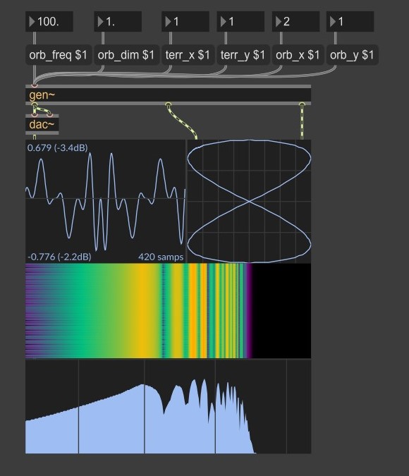
Semplice sistema di sintesi wave terrain algoritmo in GenExpr
Il terreno può essere generato tramite funzioni matematiche, algoritmi procedurali, dati campionati, immagini bidimensionali, e rappresenta l’elemento centrale nella definizione del timbro del sistema. Le sue caratteristiche determinano infatti la distribuzione delle armoniche, di eventuali discontinuità ed il comportamento spettrale complessivo del suono prodotto.
L’esempio più semplice di terreni generati attraverso funzioni matematiche è rappresentato dai terreni sinusoidali.
Grazie alla continuità delle funzioni sinusoidali, questo tipo di terreni genera variazioni morbide nel segnale audio, producendo in uscita timbri regolari ed armonici.
Degni di nota sono i terreni derivati da funzioni non lineari, le quali possono dare origine a regioni con curvature differenti, producendo spettri ricchi di parziali inarmoniche.
Terreno derivato da funzione non lineare
Altra importante categoria è costituita dai terreni generati attraverso algoritmi procedurali e processi stocastici. In questo caso il terreno non viene definito tramite una funzione semplice e regolare, ma dall’interazione di regole iterative, rumore o modelli pseudo-frattali. Tecniche basate su differenti forme di noise consentono di produrre superfici irregolari, caratterizzate da variazioni locali complesse e strutture asimmetriche.
Dal punto di vista acustico, questi terreni tendono a generare spettri densi e instabili, dando origine a sonorità articolate e complesse, particolarmente adatte alla musica elettroacustica, al sound design e alla sintesi sperimentale.
Una possibilità estremamente interessante consiste nell’utilizzare immagini bidimensionali o flussi video come terreno. In questo caso, la luminosità di ciascun pixel viene interpretata come altezza della superficie sonora. Un’immagine fotografica, un disegno astratto o il feed in real-time di una telecamera possono quindi diventare una sorgente timbrica, dando origine ad una forte relazione visivo-sonora.
Orbita
L’orbita rappresenta la traiettoria seguita dal puntatore di lettura sulla superficie ed influenza direttamente periodicità e articolazione ritmica oltre che il comportamento spettrale del suono.
Le traiettorie circolari rappresentano una delle configurazioni più semplici: il punto di lettura percorre continuamente un cammino chiuso attorno a una regione del terreno, attraversando la superficie con velocità costante. Questo tipo di scansione tende a produrre suoni relativamente stabili e periodici, soprattutto quando il terreno presenta strutture regolari o simmetriche.
dove ω rappresenta la velocità angolare, ovvero la frequenza, ed R il raggio dell’orbita e quindi l’ampiezza.
Il segnale risultante viene espresso dalla funzione:
Le orbite ellittiche introducono invece una maggiore varietà dinamica.
Con a ≠ da b, il movimento lungo i due assi avviene con ampiezze differenti. Il punto di lettura attraversa quindi regioni diverse del terreno con tempi variabili, generando timbri più articolati e meno prevedibili. Quando la frequenza dei movimenti sui due assi non coincide perfettamente, la traiettoria può produrre configurazioni quasi-periodiche, nelle quali il suono evolve continuamente senza ripetersi in modo identico.
Particolarmente importanti sono le orbite di Lissajous, ottenute dalla combinazione di oscillazioni sinusoidali indipendenti. La relazione tra frequenza, ampiezza e fase di queste oscillazioni può generare traiettorie di grande complessità, spesso caratterizzate da simmetrie intricate e da pattern in continua trasformazione.
dove: A e B rappresentano l’ampiezza dell’oscillazione, a e b la velocità angolare, la differenza di fase.
Consentendo di controllare sia la regolarità che la complessità del movimento, le orbite di Lissajous risultano particolarmente efficaci nell’esplorazione delle superfici wave terrain, offrendo un ottimo equilibrio tra prevedibilità e varietà timbrica.
L’aspetto più significativo della sintesi wave terrain emerge quindi dall’interazione tra morfologia del terreno e comportamento dell’orbita.
L’analisi delle diverse tipologie di terreno evidenzia come la natura della superficie influenzi direttamente le proprietà spettrali del segnale prodotto. Superfici regolari tendono a generare comportamenti più prevedibili e periodici, mentre terreni procedurali o irregolari introducono maggiore complessità timbrica e componenti inarmoniche. Analogamente, la scelta delle orbite determina il modo in cui queste caratteristiche si articolano nel tempo, influenzando il grado di periodicità, stabilità e complessità del risultato sonoro.
In conclusione, la possibilità di controllare in modo indipendente le caratteristiche della superficie e della traiettoria, con un elevato livello di dettaglio, rende questa tecnica uno strumento estremamente flessibile sia in ambito compositivo sia nella ricerca sulla sintesi digitale avanzata.
Il presente paper nasce da alcune riflessioni tecniche sviluppatesi parallelamente alle lezioni di “micro-composizione”. Il contributo si sviluppa come occasione di riflessione teorica e di chiarificazione concettuale, orientata a mettere in relazione pratiche e strumenti affrontati nell’esperienza didattica. Proprio queste occasioni di dialogo hanno reso evidente come tecniche di sintesi spesso presentate separatamente possano invece essere rilette attraverso un principio comune.
Nel confronto con gli studenti, la fase emerge spesso come uno dei parametri della sintesi sonora meno immediatamente riconoscibili rispetto ad altri elementi più evidenti sul piano percettivo, come la frequenza o l’ampiezza. Eppure, proprio la fase costituisce uno dei luoghi più fertili in cui si definisce il comportamento microscopico di un suono: il punto in cui il tempo viene organizzato nel dettaglio e trasformato in gesto acustico.-
L’obiettivo è osservare come la fase attraversi, come un filo rosso, diverse tecniche di sintesi sonora non troppo lontane tra loro. Distorsione di fase, modulazione di fase, modulazione di frequenza,pulsar synthesis e waveshaping possono infatti essere letti come differenti declinazioni di uno stesso principio generativo. Ciò che cambia di volta in volta è il modo in cui la traiettoria della fase viene modellata, perturbata o reinterpretata.
Prima di addentrarci in configurazioni più articolate, può essere utile richiamare casi fondamentali da “ripasso matematico”: situazioni ben note sul piano della funzione esponenziale, ma che, applicate alla traiettoria della fase, acquistano una precisa rilevanza sonora.
Distortione di fase
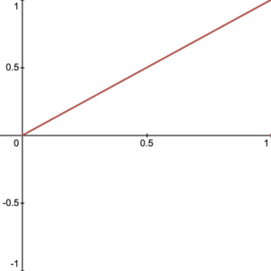
Un primo esempio particolarmente chiaro è offerto dalla distorsione di fase. Qui si può immaginare la fase come una rampa lineare che cresce uniformemente da 0 a 1, prima ancora di essere convertita nell’escursione completa da 0 a . La rampa rappresenta quindi un tempo normalizzato, distribuito in modo uniforme lungo un ciclo.
La forma più semplice di fase può ovviamente essere descritta come:
Fase normalizzata
Fase normalizzata, in rosso
Output, in nero
Su questa traiettoria lineare si può intervenire alterandone l’andamento, cioè distorcendo la fase, progettando il modo in cui il suono attraverserà il proprio ciclo: decidere dove accelerare, dove rallentare, dove concentrare o distribuire l’energia.
Osservando la trasformazione della fase, emerge come il parametro di possa essere considerato entro le tre seguenti aree operative, ciascuna capace di produrre una diversa organizzazione temporale del ciclo: maggiore di 1, tra 0 e 1 e negativo.
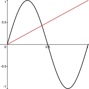
maggiore di 1
Si tratta di una delle trasformazioni più immediate.
Fase normalizzata, in rosso
Output, in nero
Il tempo interno al ciclo viene redistribuito. Quando questa traiettoria viene poi utilizzata per leggere una sinusoide, il risultato non è soltanto una variazione grafica della curva, ma una diversa articolazione del moto oscillatorio: la sinusoide viene “percorsa” con velocità variabile all’interno del ciclo, generando un differente profilo timbrico.
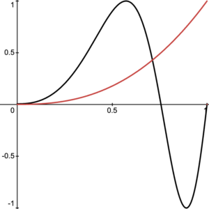
tra 0 e 1
I numeri elevati a un esponente tra zero e uno si calcolano estraendo una radice. Esempio:
Con fase normalizzata tra 0 e 1 – ed anch’esso tra 0 e 1 – la rampa inverte la curvatura:
Fase normalizzata, in rosso
Output, in nero
negativo
Una terza area riguarda i valori negativi. In questo caso il comportamento della funzione cambia in modo più radicale. Elevare una quantità compresa tra 0 e 1 a un esponente negativo equivale infatti a calcolarne il reciproco:
Ne derivano andamenti che crescono rapidamente già nelle vicinanze dello zero. Alcuni esempi rendono il fenomeno immediatamente visibile:
Più si avvicina a zero, più il valore risultante di cresce rapidamente:
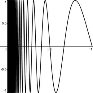
Versione non wrapped della funzione
Dal punto di vista sonoro, tali configurazioni possono produrre sfumature glitch con aliasing. Quest’ultimo, pur essendo un effetto da limitare in innumerevoli casi, può essere impiegato creativamente.
Per rendere più leggibile il comportamento della fase in questa terza area, e al tempo stesso ridurre al minimo le problematiche legate all’indeterminatezza che si verifica quando lo zero viene elevato a un esponente negativo, può essere introdotto un piccolo offset numerico (0.001 nella funzione sottostante). Inoltre, applicando una funzione di wrap mediante l’operazione ‘modulo’, è possibile osservare con maggiore chiarezza il riavvolgimento ciclico della fase all’interno del grafico.
La funzione può quindi essere espressa come:
In questa forma la traiettoria resta confinata entro il dominio normalizzato tra 0 e 1, rendendo immediatamente visibile sia la deformazione della rampa sia il punto in cui essa si riavvolge. L’osservazione grafica di questa curva, accostata alla sinusoide risultante, permette di mettere in relazione diretta il profilo della fase e la trasformazione dell’onda che ne deriva.
Versione wrapped della funzione
Fase con wrap, in rosso
Output, in nero
Output
Fase: da distorsione a modulazione
Che differenza c’è tra distorcere e modulare? In generale, distorcere significa alterare direttamente la forma di un segnale o di una sua rappresentazione, modificandone la struttura senza che sia necessariamente presente un controllo esterno variabile nel tempo. Modulare, invece, significa utilizzare un segnale per controllare nel tempo il comportamento di un altro segnale, introducendo una variazione dinamica che può essere lenta o rapida. Nel caso della fase, la distorsione consiste nel deformarne direttamente l’andamento all’interno del ciclo, mentre la modulazione consiste nel farla variare attraverso l’azione di una modulante. Nonostante questa distinzione concettuale, entrambe le tecniche appartengono alla più ampia famiglia delle manipolazioni della fase e possono produrre risultati spettrali sorprendentemente simili, pur partendo da principi operativi differenti.
Nella distorsione di fase la rampa viene dunque piegata o riavvolta modificandone l’andamento complessivo. Nella modulazione di fase (da qui in poi PM), invece, la progressione lineare resta percepibile ma è attraversata da una perturbazione oscillatoria: la fase viene ondulata periodicamente, generando accelerazioni e rallentamenti distribuiti lungo il ciclo.
La sola traiettoria di fase può essere descritta come:
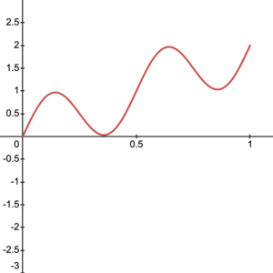
La componente lineare mantiene la progressione regolare della fase, mentre il termine sinusoidale introduce una deviazione ciclica. Il parametro controlla l’ampiezza di questa deviazione; ne determina invece la periodicità all’interno dell’intervallo osservato.
Solo fase modulata
Indice e frequenza modulante
Nelle rappresentazioni del presente articolo, non indica il tempo fisico ma una fase normalizzata compresa tra 0 e 1, utilizzata per evidenziare il ruolo della fase come materiale comune alle diverse tecniche di sintesi.
Dal punto di vista grafico, la traiettoria non appare più come una semplice rampa, ma come una linea che conserva il proprio andamento ascendente mentre viene deformata da ondulazioni regolari. È proprio questa oscillazione locale della fase a determinare la trasformazione sonora successiva.
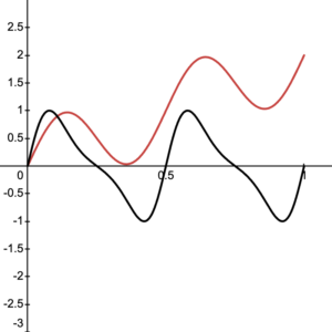
Phase Modulation
Solo fase modulata, in rosso
Output, in nero
Indice, portante e modulante
Qui rappresenta la frequenza portante, mentre il termine modulante altera continuamente la velocità istantanea con cui la sinusoide viene attraversata.
Nella manualistica della musica elettronica questo stesso principio viene spesso descritto anche attraverso la modulazione di frequenza. Le due formulazioni (modulazione di frequenza e di fase) conducono infatti al medesimo risultato sonoro e generano lo stesso contenuto spettrale se la modulante è sinusoidale. La differenza riguarda soprattutto il modo in cui il processo viene concettualizzato e implementato.
La lettura attraverso la fase evidenzia la deformazione diretta della traiettoria interna al ciclo; quella attraverso la frequenza descrive invece la variazione istantanea della velocità con cui la fase viene percorsa. In molti strumenti basati su wavetable synthesis la prima prospettiva risulta particolarmente immediata: il materiale sonoro viene letto all’interno di una tabella mentre il puntatore di fase, anziché procedere linearmente, viene deformato o ondulato secondo funzioni di controllo.
Ciò che accomuna entrambe le tecniche è il ruolo centrale della fase come spazio di micro-composizione: il timbro nasce dal modo in cui viene progettato e perturbato il percorso interno al ciclo, prima ancora che questo diventi suono udibile.
Per rendere più evidente questa relazione, nelle seguente figura sono messe a confronto PM e FM realizzate in Max:
Nella PM, il segnale modulante agisce direttamente sulla fase dell’oscillatore portante, aggiungendo e sottraendo radianti al suo percorso interno. Nella FM, invece, il segnale modulante viene convertito in una deviazione della frequenza istantanea.
Affinché una patch di FM risulti perfettamente equivalente alla formulazione matematica osservata qualche paragrafo sopra — che coincide con la classica espressione della PM — è necessario che l’indice di modulazione venga moltiplicato per la frequenza modulante . Questo prodotto viene poi moltiplicato per l’uscita dell’oscillatore modulante, ottenendo così la deviazione di frequenza da sommare alla portante:
Nel confronto mostrato in figura, la frequenza modulante è fissata a 250 Hz, la portante a 2000 Hz e l’indice a 2.
Nella PM l’indice agisce come deviazione di fase espressa in radianti: il modulatore anticipa e ritarda continuamente il percorso della portante di ±2 radianti alla frequenza di 250 Hz.
Nella FM, lo stesso valore numerico determina invece la deviazione istantanea di frequenza secondo la relazione:
Perciò, con:
si ottiene:
La frequenza istantanea oscilla quindi tra 2000 + 500 e 2000 – 500 Hz.
Nella modulazione di fase i parametri e , pur intervenendo sulla fase, ne modificano continuamente la velocità di avanzamento: la deviazione resta dunque una deviazione di fase, ma produce allo stesso tempo una variazione della velocità istantanea del phasor, quindi una deviazione di frequenza misurabile anch’essa in Hertz.
La FM può essere letta, in questa prospettiva, come una variante didatticamente efficace della PM: rende immediatamente percepibile la relazione tra indice, frequenza modulante e deviazione espressa in Hertz, offrendo una formulazione semplice e intuitiva del fenomeno. John Chowning sviluppò e formalizzò storicamente questo principio come frequency modulation, mettendo in evidenza il controllo delle deviazioni di frequenza e le loro conseguenze spettrali. Nella pratica dei sintetizzatori digitali successivi, tuttavia, l’implementazione avviene spesso attraverso la PM: è il caso, ad esempio, dello Yamaha DX7, storicamente associato alla FM ma basato internamente sulla modulazione della fase. La distinzione resta quindi utile sul piano teorico e descrittivo, mentre sul piano sonoro e operativo i due modelli tendono spesso a convergere quando, come già detto, la modulante è sinusoidale. Con modulanti di diversa natura, FM e PM possono invece dar luogo a comportamenti differenti, come si noterà nel prossimo contributo.
Il termine “Composizione Elettroacustica” genera talvolta equivoci tra musicisti chenon hanno ancora avuto occasione di confrontarsi con le discipline legate alla musica elettronica. Analoghe incomprensioni possono naturalmente emergere anche al di fuori dell’ambito musicale. Lo scopo di queste riflessioni non è proporre una definizione definitiva dell’argomento, ma offrire alcuni strumenti utili per comprenderne meglio il significato, l’evoluzione storica e le principali aree di interesse.
Definire oggi il concetto di Composizione Elettroacustica non è immediato. Nel corso degli anni questo termine ha assunto significati diversi, e una certa ambiguità che ancora lo accompagna deriva probabilmente proprio dalla natura storicamente mutevole dell’idea di musica elettronica e dei modelli didattici ad essa associati. Tra le discipline consolidate all’interno del Conservatorio, la composizione elettroacustica è quella che negli ultimi anni ha più subito trasformazioni continue: tecniche, estetiche e culturali. La sua identità non si è definita come un sistema stabile e immutabile, ma come un ambito in costante ridefinizione.
Nel senso più comune, la composizione elettroacustica viene spesso intesa come l’insieme delle pratiche musicali prodotte mediante strumenti e tecnologie elettroniche o digitali. Una simile definizione, tuttavia, appare eccessivamente ampia e rischia di includere contesti estremamente diversi tra loro, fino a perdere ogni specificità. Se si volesse invece individuare un nucleo più preciso del termine, si potrebbe affermare che la composizione elettroacustica riguarda quelle forme musicali in cui la presenza della tecnologia non costituisce soltanto un mezzo di produzione, ma diviene parte percepibile e strutturale del risultato sonoro. In altri termini, non si tratta soltanto di utilizzare strumenti tecnologici per comporre: si tratta di una musica nella quale il rapporto con la tecnologia entra a far parte dell’identità stessa del suono e della sua organizzazione.
Anche questa definizione, tuttavia, richiede ulteriori precisazioni. Il panorama contemporaneo mostra infatti come il suono tecnologico attraversi ormai una quantità vastissima di linguaggi e generi musicali. Per questo motivo può risultare utile ricondurre il concetto di composizione elettroacustica a due nuclei creativi fondamentali: quello della micro-composizione e quello della macro-composizione.
Con il termine micro-composizione si intende il lavoro creativo che interviene direttamente sulla costruzione del suono: la sua sintesi, la sua trasformazione, la sua elaborazione timbrica e morfologica. Rientrano in questo ambito, ad esempio, la progettazione di processi granulari, la definizione di algoritmi e funzioni personalizzate per la generazione sonora, la costruzione di sistemi di controllo dettagliati, l’elaborazione di modelli di trasformazione del timbro. In ambito contemporaneo molte di queste pratiche vengono comunemente ricondotte al termine sound design; tuttavia la nozione di micro-composizione pone l’accento in modo più specifico sulla dimensione compositiva del dettaglio sonoro, evidenziando come il lavoro sul suono stesso costituisca già un atto creativo strutturale.
Micro-composizione su Max
La macro-composizione riguarda invece l’organizzazione dei materiali nel tempo e nello spazio, ovvero ciò che per tradizione chiamiamo “composizione musicle”: la disposizione orizzontale e verticale degli eventi sonori, la costruzione di sequenze, ritmi, dinamiche, densità, intervalli, armonie e relazioni formali. È la dimensione nella quale il materiale prende forma come discorso musicale e viene articolato all’interno di una struttura più ampia. Se la micro-composizione agisce all’interno del suono, la macro-composizione ne organizza il comportamento e il significato su scala più estesa.
Macro-composizione
Un ulteriore elemento di complessità riguarda il rapporto con i generi musicali. Negli ultimi decenni il panorama sonoro si è progressivamente trasformato, e la distinzione rigida tra repertori “alti” e “bassi”, almeno sul piano della riflessione critica e della produzione creativa, si è fortemente attenuata. Se agli esordi la musica elettronica era legata soprattutto alle avanguardie storiche e ai contesti accademici di ricerca, oggi l’ambito elettroacustico si estende attraverso territori estremamente eterogenei. Ne fanno parte pratiche legate alla tradizione acusmatica o spettrale, ma anche forme sviluppatesi in contesti indipendenti e underground — come IDM, glitch, ambient elettronica, experimental techno e molte altre — fino a linguaggi più vicini alla produzione elettronica di larga diffusione.
In questa prospettiva il compito dell’ambito accademico non consiste tanto nel delimitare rigidamente un genere, quanto nel costruire uno spazio di conoscenza trasversale capace di attraversare linguaggi differenti, individuandone principi comuni e mettendone in luce i processi creativi fondamentali. Il centro della riflessione non coincide necessariamente con uno stile specifico, ma con il rapporto creativo tra suono, tecnologia e pensiero compositivo.
Alla distinzione tra “micro” e “macro-composizione” può corrispondere, volendo, anche una distinzione tra micro-analisi e macro-analisi. La prima si concentra sull’osservazione dei fenomeni sonori e dei processi creativi che li generano — timbro, spettro, sintesi, filtraggio e trasformazioni del suono — mentre la seconda considera aspetti più ampi come la forma, il ritmo, la distribuzione dei materiali e l’organizzazione complessiva del discorso musicale. Pur distinguibili sul piano teorico, queste due prospettive risultano nella pratica strettamente connesse, poiché le caratteristiche del singolo suono possono influenzare la forma dell’opera, così come le scelte formali possono orientare la progettazione del materiale sonoro.
Definire la composizione elettroacustica significa allora riconoscere una pratica musicale che mette in relazione tecnologia e creatività su più livelli: nella costruzione del dettaglio sonoro e nella forma complessiva; nella ricerca analitica e nell’invenzione; nella continuità con il repertorio storico e nell’apertura verso i linguaggi emergenti. Ambienti come Max o simili, nati proprio per offrire strumenti di progettazione e sperimentazione sonora, rappresentano in modo emblematico questa prospettiva di micro-composizione: luoghi nei quali il gesto tecnico può coincidere con il pensiero creativo.
John Chowning’s Stria, a case study from the TaCEM project
The TaCEM project (Technology and Creativity in Electroacoustic Music) has investigated the relationship between technological innovation and compositional processes on the basis of nine case studies, including John Chowning’s Stria (1977). Each case study involved researching the historical and contextual background of the work, emulating the technology used to create it and analyzing its musical structure. For each of these electroacoustic works, a specially designed software package has been developed, forming an important part of the project outcome. If Stria, as a classic work of the electroacoustic repertoire, has been much written about, the study presented in this article is distinctive in that the software enables to present the results of this research in an interactive and aural form: its users can engage directly with the structure of the work and the techniques and processes used by Chowning to compose it. This article presents this interactive aural analysis approach, its application to Stria, and the interactive resources embedded into the resulting software.
INTRODUCTION
Researching music in which technology plays an integral part in the creative process presents particular challenges as well as opportunities for musicologists. This is particularly the case in works where technology has changed the way in which the music is conceived and where detailed knowledge of the technology therefore plays a crucial part in developing a full understanding of the creative process. The task becomes more difficult in cases the technology used to produce the original work no longer exists. But even where the technology does exist, it may not be easily available to a wide range of researchers or may not be in a form they will find accessible. Written documentation and description can give some indication of the technical system but is no substitute for the knowledge that can be gained from exploring a working version, trying out different options and hearing the results in a hands-on environment. And this is also especially important in connecting technical investigation with research into the musical structure of a work, exploring how the technical and creative interact. These relationships are crucial to a well-informed understanding of the works concerned, not least in terms of how the associated technologies have influenced the creative process. Although the importance of thus engaging with the Techné or art of bringing forth such works via a technical medium has been recognized for many years – see for example articles written by Di Scipio in 1995 [1] and Manning in 2006 [2] – the development of suitable tools for such investigations has still a long way to go. In the TaCEM project, Technology and Creativity in Electroacoustic Music1, a 30-month project funded by the Arts and Humanities Research Council in the UK, the authors have attempted to address these issues by creating interactive software to help investigate both the musical structure of works and the processes that led to their creation. This approach builds on Clarke’s earlier work on Interactive Aural Analysis [3]. The main output of our project will be a book with substantial accompanying software. John Chowning’s Stria is one of nine case studies examined for the project. Each case study involves researching the background to the work, emulating the technology used to create it and analyzing its musical structure2. With each of our case studies, a specially designed software package forms an important part of the outcome. Stria is a classic of the electroacoustic repertoire and, as such, much has previously been written about it, most notably in a 2007 edition of the Computer Music Journal [5, 6, 7, 8]3. What makes our study distinctive is the way software enables us to conduct our research and present it from an interactive aural perspective, and in so doing explores the characteristics of the works being studied in greater depth. We can investigate technological aspects by working with models that emulate the processes employed and comparing our results with the original. We can examine the significance of the choices the composer made in shaping the work by trying out alternative parameter settings within their creative environment and evaluating the results aurally. We have drawn on previous work on Stria and have also benefitted greatly from the help and advice of John Chowning himself. Video interviews we conducted with the composer during a visit to Stanford form another important aspect of our software package, adding a poietic perspective. Another very significant aspect of our study, one not represented in this paper, is contextual research, placing the work in its wider technical and musical context. The purpose of this paper is not to give a full analysis of Stria (that will appear in the book arising from the project) but rather to provide an introduction to our working methods together with the software and to demonstrate and discuss the advantages of approaching this type of repertoire through the use of interactive resources.
OVERVIEW OF THE SOFTWARE
The software for our study of Stria incorporates various different components, combining technical study, musical analysis and video interviews with the composer. The associated text, in a book chapter, provides further contextual information and more detailed explanation of the technical and creative issues presented in the software. To gain most from these materials, the text and software need to be studied in tandem and the chapter will contain links to video demonstrations of the software to facilitate this articulation. The software package for Stria comprises seven interactive explorers, interleaved with related video extracts from our interviews with the composer. Figure 1 provides an overview of the TaCEM software for the study of Stria.
Figure 1. Overview of the TaCEM software for the analysis of Stria. On the left side is an Interactive Aural Presentations bar, enabling the user to navigate through interactive explorers and videos. The central canvas is the main interactive workspace for a given presentation (here, presentation 1: the Interactive Structural Chart representing the global structure of Stria). On the right side is the presentation inspector, providing access to further options for advanced visualization and playback.
INTERACTIVE EXPLORERS
The first interactive presentation is an Interactive Structural Chart. As seen in figure 1 above, this chart sets out all the “elements” that comprise Stria in temporal order from left to right along the horizontal axis. “Element” is the term Chowning uses for the smallest component of the work, roughly equivalent to a “note” in a traditional score. These elements come together to form the “events” which in turn build up the six “sections” of Stria. In our interactive structural chart, individual elements can be heard by clicking on them and, alternatively, the whole texture at any point in the work may be played. The criteria used to order the vertical arrangement of the elements can be changed by the user from a menu in the presentation inspector, on the right side of the window. The default option, as on figure 1, simply presents the elements in polyphonic order, so that overlapping elements are stacked vertically. However, any of the individual synthesis parameters used in the creation of Stria may determine the vertical arrangement. For example, the carrier frequency, either of the two modulation frequencies, the reverberation amount or the distance factor can be represented on the vertical axis. In this way, an overview of the shape of the work can be seen from many different perspectives. Importantly, because of the interactive aural nature of the chart, seeing can be linked directly to hearing. The sounds presented in this chart are synthesized live by the emulation software and this means that it is possible in listening to examples from this chart to bypass certain aspects of the synthesis process so that their significance and contribution to the overall sound can be perceived and understood. The aspects that can be deactivated are the operation of the two modulators, the skew (a small dynamic pitch variation adding richness to the overall sound) and the reverberation. Interestingly, the shape of the work as shown (and heard) by this interactive chart, for example when ordered by carrier frequencies (figure 2), does not correspond neatly to the “V”-shape frequently portrayed, for example on the cover of the aforementioned 2007 issue of the Computer Music Journal (figure 3). It is not clear what specific data, whether parameter data inputted or outputted results, was used to draw this shape, though it does correspond to the composer’s own description of the shape of the work (for example, in our interviews with him)4. In terms of the parameters shown in our Interactive Structural Chart, the form of the work, although generally following this shape, is a far more complex interaction with many contributing factors. Being able to identify and explore such issues is one of the advantages of working directly with an interactive emulation of the technology and with flexible visualization features.
Figure 2. Elements of Stria sorted vertically by carrier frequenciesFigure 3. The shape of Stria as depicted on the cover of the 2007 issue of the Computer Music Journal
The next group of interactive explorers relate to the synthesis method used in the work. This is the frequency modulation (FM) method, famously developed by Chowning himself and later used in many different software packages and patented for use in commercial synthesizers by Yamaha. Three interactive explorers introduce the reader in stages to this synthesis method and how it is used in Stria. Firstly, the basic principles of FM are introduced followed by the more complex, two-modulator version of FM used in Stria. Our interactive software enables users to try out the technique for themselves either using examples of the input data from Stria itself or inputting their own settings. The software has an option to display numerical data about the frequencies generated by the modulation process (the frequencies of the sidebands), as well as showing them graphically (figure 4). Displaying this data numerically is useful in analyzing the often complex results arising from two-modulator FM synthesis. Indeed, it is particularly helpful in exploring the significance of the ratio used by Chowning in this work (the Golden Mean) and what this means in terms of the timbres generated.
Figure 4. Two-modulator, one-carrier frequency modulation with graphical and numerical representations of sideband frequencies
The next interactive FM explorer demonstrates the potential of dynamic evolution of timbres in FM synthesis using envelopes to shape parameters (figure 5).
Figure 5. Interactive explorer of dynamic FM. The envelopes are applied to the overall amplitude, to the skew, and to the two modulation indexes.
The software displays the envelopes and these can be changed interactively to facilitate greater understanding of their importance through direct aural experience.
A further interactive explorer builds on the FM examples already introduced and extends them to include all the parameters involved in defining an element in Stria, including spatialization. In this explorer, the user can shape individual elements using the same parameters as used to control the synthesis engine in Stria. These synthesis parameters are grouped according to the following categories: time parameters, frequency parameters, modulation parameters, spatialization, and envelope functions (figure 6). A two-dimensional surface enables to set the amplitudes of the four output channels by providing an angle directly. The envelope layout highlights Chowning’s specific use of the terms “attack” and “decay” in Stria: the attack setting, in seconds, determines the time to go through the first quarter of the envelopes. Likewise, the decay setting determines the time to go through the last quarter of the envelopes. Interacting with this explorer reveals, by modifying the duration, attack and decay parameters and watching the playhead on the envelope panels, the non-linear indexing of Chowning’s functions.
Figure 6. Interactive explorer for the definition of one element according to synthesis parameters
In the composition of Stria itself, Chowning did not shape the elements individually. Instead, the composer programmed an algorithm to do this work, with him inputting data to higher-level parameters he created to define the structure of a whole event. Unlike our emulation, Stria was produced using software that did not operate in real-time. Indeed, there were significant delays waiting for sounds to be generated. In our interviews, the composer described the advantages he found in working in this way: it gave him time to reflect and plan at a time when many of the ideas and techniques he was employing were new and unexplored. Furthermore, the piece was not produced directly in a single process but in two successive stages. The first stage, using the program the composer himself constructed in SAIL (Stanford Artificial Intelligence Language), used algorithms to generate the data defining the elements comprising each event in the work. To realize these elements in sound, a second stage was then required, in which the data generated by the SAIL algorithm was imported into Music 10 as score data and the sounds were then generated (again, not in real-time). The Music 10 orchestra for Stria remains fixed throughout the work and generates sounds using the two-modulator FM synthesis algorithm mentioned above, with the addition of global reverberation and four-channel spatialization.
In our software emulation of the whole process, these two separate stages are combined into one and the whole operation is run in real-time. Despite the benefits Chowning found in not working in real-time when composing the work, in the context of studying the music and its technical and creative processes, real-time has the advantage of allowing readers to engage more directly with the music as sound and helps develop an understanding of the aural significance of particular parameters and of the settings chosen by the composer. As a default, users are provided with the original settings Chowning used in Stria, but they may also input their own alternatives, either using an emulation of the composer’s original interface, inputting data one item at a time in response to onscreen prompts (figure 7), or using a more modern graphical interface (figure 8). Chowning’s original SAIL program takes the user parameters and inputs the data from these into an algorithm that calculates the individual elements for a particular event. The algorithm is determinist: inputting the same data will always result in rigorously the same outcome. To the novice user, the significance of the input parameters may not be immediately obvious, especially when encountered in the original command-line format. This is particularly the case as some aspects of the resulting sound (for example the fundamental pitch of an element) are influenced by the interaction of several different parameters (in the case of the fundamental frequency these include range, division of this range, multiplier, etc.). To make this easier to understand and to show the effect of changing parameter settings, our software emulation incorporates visual displays of the parameters and the resulting elements. Furthermore, to facilitate conceptual understanding of how Chowning’s design of the algorithm enables him to shape the music, the emulation includes the option of showing visually how an event is formed step by step, starting with temporal definitions for events and the elements they contain (for the event: start time, duration, attack duration5; for the elements: start positions and durations), then frequency definitions (base frequency, frequency space), followed by modulation parameters, element attacks and decays, and spatialization. In this way, the creative and technical thinking behind the algorithm is revealed.
Figure 7. Emulation of the SAIL terminal interface to create one event in StriaFigure 8. Graphical User Interface for the creation of one event
VIDEOS
Our analytical and technical investigations into Stria are complemented by poietic material in the form of interviews with the composer that we conducted over three days in March 2015. Extracts from these interviews are interleaved with the software presentations so that topics explored through the software appear alongside related discussions with the composer (figure 9). These interviews will also be referenced and in part transcribed in the accompanying book text. The topics covered by the interviews range from specific issues relating to the composition of Stria to general discussion of the FM synthesis technique, to much broader topics concerning the Chowning’s career and his more recent compositional concerns.
Figure 9. Filmed interview with John Chowning at CCRMA in Stanford (March 2015), as embedded amongst the presentations in the TaCEM software
In total there are nine videos of varying length. They are entitled according to the following topics: The shaping of Stria; Pioneering digital spatialization and Frequency Modulation; Musical uses of Frequency Modulation; Approaches to programming (SAIL and Max); The different versions of Stria; Encounters and interactions with JeanClaude Risset; Academic and commercial impact of Chowning’s work; Chowning’s compositional process and career; and From Stria (1977) and Phoné (1981) to Voices (2005). In this way, the detailed and specific study of Stria and the technology behind it can be related to the composer’s creative intentions and to the broader picture of his contribution to the development of computer music.
CONCLUSION
Combining software with written text and filmed interviews enables those who use our resources to gain a deeper understanding of a work, in this case Stria, than would be possible using text alone:
– they can discover the potential of synthesis techniques by working with them rather than just reading about them as theory;
– they can explore the musical shape of works as sound;
– they can hear the musical impact of the choices the composer made;
– they can see and hear composers giving their own accounts of the works and their broader context.
Especially as, over time, many of the original technical resources employed in particular works become obsolete, our approach of creating good approximations to these technologies helps to ensure that detailed understanding of those technologies and of what it was like to work with them is preserved. Furthermore, the articulation of software, text and interviews helps to preserve and transmit to new generations lessons learnt about the successful combining of technical knowledge and creative inspiration. Indeed, in trialing these materials in a pedagogic context we have discovered their potential for bringing together aspects of music technology teaching that are more often kept as isolated units: students can learn about the history of computer music, they can explore techniques (e.g. FM synthesis), they can investigate how a particular work is structured musically and, using our emulation software if they wish, they can try out creative ideas inspired by all that they have learnt, producing their own compositional sketches. In a digital age, surely it does not make sense to rely solely on written text to try and convey matters relating to sound, complex technology, and creativity. Engaging with this repertoire aurally and interactively adds an important additional dimension to the mode of enquiry and significantly enriches what can be conveyed and learnt.
[1] A. Di Scipio, “Centrality of Techné for an Aesthetic Approach on Electroacoustic Music”, Journal of New Music Research, vol. 24, no. 4, 1996, pp. 369- 383. [2] P. Manning, “The significance of Techné in Understanding the Art and Practice of Electroacoustic Composition”, Organised Sound, vol. 11, no. 1, 2006, pp. 81-90. [3] M. Clarke, “Analysing Electroacoustic Music: an Interactive Aural Approach”, Music Analysis, vol. 31, no. 3, 2012, pp. 347-380. [4] M. Clarke, F. Dufeu, P. Manning, “From Technological Investigation and Software Emulation to Music Analysis: An integrated approach to Barry Truax’s Riverrun”, Proceedings of the 2014 International Computer Music Conference / Sound and Music Computing conference, Athens, 2014, vol. 1, pp. 201-208. [5] M. Meneghini, “An Analysis of the Compositional Techniques in John Chowning’s Stria”, Computer Music Journal, vol. 31, no. 3, 2007, pp. 26-37. [6] L. Zattra, “The Assembling of Stria by John Chowning: A philological investigation”, Computer Music Journal, vol. 31, no. 3, 2007, pp. 38-64. [7] K. Dahan, “Surface Tensions: Dynamics of Stria”, Computer Music Journal, vol. 31, no. 3, 2007, pp. 65-74. [8] O. Baudouin, “A Reconstruction of Stria”, Computer Music Journal, vol. 31, no. 3, 2007, pp. 75-81. [9] B. Bossis, “Stria de John Chowning ou l’oxymoron musical : du nombre d’or comme poétique”, in É. Gayou (ed.), John Chowning. Portraits Polychromes, Paris, Ina-GRM, TUM-Michel de Maule, 2005, pp. 87-105. [10] C. Dodge, T. Jerse, Computer Music. Synthesis, Composition, and Performance, 2nd ed., London and New York, Schirmer, 1997.
Another “V”-shape can be found in [10], p. 137. As Zattra notes in [6], p. 45, “Dodge and Jerse consider this [latter] figure a sketch of the shape (without any claim to be precise in details) of the 18-minute piece”. ↩︎
In the terminology of Stria and its programs, the attack duration of an event is the duration within which new elements can be generated. If an event has a duration of 60 seconds and an attack duration of 30 seconds, no new element will appear during the second half of the event. ↩︎